In this document, we provide all steps and R codes required to estimate the effect of heat waves on the number of years of life lost (YLL) using cardinality matching. The implementation is done with the package designmatch. Giancarlo Visconti and José R. Zubizarreta (2018) provide a great tutorial to learn the method. As for other matching procedures, we also rely on the cobalt package for checking covariate balance.
Should you have any questions, need help to reproduce the analysis or find coding errors, please do not hesitate to contact us at leo.zabrocki@gmail.com.
Required Packages and Data Loading
To reproduce exactly the cardinality_matching.html document, we first need to have installed:
- the R programming language
- RStudio, an integrated development environment for R, which will allow you to knit the cardinality_matching.Rmd file and interact with the R code chunks
- the R Markdown package
- and the Distill package which provides the template for this document.
Once everything is set up, we load the following packages:
# load required packages
library(knitr) # for creating the R Markdown document
library(here) # for files paths organization
library(tidyverse) # for data manipulation and visualization
library(broom) # for cleaning regression outputs
library(designmatch) # for optimal cardinality matching
library(gurobi) # for fast optimization solving
library(cobalt) # for assessing covariates balance
library(lmtest) # for modifying regression standard errors
library(sandwich) # for robust and cluster robust standard errors
library(Cairo) # for printing custom police of graphs
library(DT) # for displaying the data as tables
In this document, we improve the performance of cardinality matching by using the Gurobi optimization solver. To install the solver, you need (i) to obtain a free academic licence, (ii) install Gurobi on your computer and (iii) the R package gurobi. This vignette guides your through these three steps.
We then load our custom ggplot2 theme for graphs:
We finally load the data:
# load the data
data <-
  readRDS(here::here("inputs", "1.data", "environmental_data.rds")) %>%
  # define year as factors
  mutate(year = as.factor(year)) %>%
  # create dummies for month and year
  fastDummies::dummy_cols(., select_columns = c("month", "year")) %>%
  drop_na()
As a reminder, there are 122 days where an heat wave occurred and 1251 days without heat waves.
Cardinality Matching
Cardinality matching is a relatively new method to find the largest sample size that meets specific constraints on covariate balance (Giancarlo Visconti and José R. Zubizarreta, 2018). This method avoids the cumbersome process of checking, often through several iterations, that a matching procedure leads to the desired covariate balance.
Concretely, we can ask the algorithm to find the pairs of treated and control units for which the standardized difference for each covariate is less than a specific value. Here, we require that the standardized difference in covariates should be less than 0.01, so that the matched sample is very balanced.
Once we have found the largest sample of pairs that meet our balance constraints, we can rematch the matched sample to find pairs that are very similar according to a covariate that is predictive of the outcome of interest. This rematching helps reduce the heterogeneity in pair differences: the estimated treatment effect will be more precise and less sensitive to hidden bias (a point which is beyond the scope of this tutorial but which is explained in greater details in Chapter 16 of Design of Observational Studies by Paul Rosenbaum). Here, we rematch our matched sample according to the the June indicator.
Matching to Find the Largest Sample Meeting Balance Constraints
In this section, we implement cardinality matching to find the largest sample of treated and control pairs for which the standard difference in each covariate is less than 0.01.
First, the designmatch package requires that the treatment variable is arranged in the decreasing order:
# specify the ordering of the treatment variable
data <- data %>% mutate(heat_wave = ifelse(heat_wave==TRUE, 1, 0)) %>% arrange(-heat_wave)
We then select the covariates we want to balance: lags of heat wave indicator, relative humidity, lags of ozone and nitrogen dioxide concentrations, and calendar indicators.
# select covariates
data_covs <- data %>%
  dplyr::select(
    heat_wave_lag_1:heat_wave_lag_3,
    humidity_relative,
    o3_lag_1:o3_lag_3,
    no2_lag_1:no2_lag_3,
    weekend,
    month_august:year_2007
  ) %>%
  as.data.frame()
We implement cardinality matching using the bmatch() function and require that the standardized mean differences between treated and control units should be less than 0.01:
# set solver options
t_max = 60*30
name = "gurobi"
approximate = 1
solver = list(name = name, t_max = t_max, approximate = approximate, round_cplex = 0, trace = 1)

# implement cardinality matching
card_match_1 <- bmatch(
  data$heat_wave,
  dist_mat = NULL,
  subset_weight = NULL,
  mom = list(
    covs = data_covs,
    tols = absstddif(data_covs, data$heat_wave, .01)
  ),
  solver = solver
)
  Building the matching problem...
  Gurobi optimizer is open...
  Finding the optimal matches...
Gurobi Optimizer version 9.5.1 build v9.5.1rc2 (win64)
Thread count: 4 physical cores, 8 logical processors, using up to 8 threads
Optimize a model with 1437 rows, 152622 columns and 10073052 nonzeros
Model fingerprint: 0x91ab9bca
Coefficient statistics:
  Matrix range     [3e-05, 8e+01]
  Objective range  [1e+00, 1e+00]
  Bounds range     [1e+00, 1e+00]
  RHS range        [1e+00, 1e+00]

Concurrent LP optimizer: dual simplex and barrier
Showing barrier log only...

Presolve removed 1 rows and 0 columns (presolve time = 5s) ...
Presolve removed 1 rows and 0 columns
Presolve time: 7.59s
Presolved: 1436 rows, 152622 columns, 9920430 nonzeros

Ordering time: 0.02s

Barrier statistics:
 AA' NZ     : 2.411e+05
 Factor NZ  : 2.793e+05 (roughly 60 MB of memory)
 Factor Ops : 5.866e+07 (less than 1 second per iteration)
 Threads    : 3

                  Objective                Residual
Iter       Primal          Dual         Primal    Dual     Compl     Time
   0  -1.75201140e+05  0.00000000e+00  1.85e+06 2.50e-01  6.06e+00    10s
   1  -1.01598231e+05 -8.05818950e+02  1.07e+06 3.47e-02  3.35e+00    10s
   2  -3.58256029e+03 -8.24850335e+02  3.64e+04 3.33e-16  1.23e-01    11s
   3  -4.64537527e+02 -4.92640892e+02  3.61e+03 4.44e-16  1.60e-02    12s
   4  -2.29317837e+02 -3.19377401e+02  1.13e+03 3.33e-16  5.84e-03    13s
   5  -1.51380469e+02 -2.64535472e+02  3.34e+02 3.33e-16  2.76e-03    14s
   6  -1.21788751e+02 -1.58283408e+02  2.66e+01 5.00e-16  5.45e-04    15s
   7  -1.22139401e+02 -1.49864332e+02  2.06e+01 3.89e-16  4.10e-04    16s
   8  -1.22608364e+02 -1.43936449e+02  1.74e+01 2.78e-16  3.16e-04    17s

Barrier performed 8 iterations in 17.08 seconds (8.42 work units)
Barrier solve interrupted - model solved by another algorithm


Solved with dual simplex
Solved in 1191 iterations and 17.15 seconds (9.11 work units)
Optimal objective -1.220000000e+02
  Optimal matches found
Gurobi Optimizer version 9.5.1 build v9.5.1rc2 (win64)
Thread count: 4 physical cores, 8 logical processors, using up to 8 threads
Optimize a model with 1373 rows, 152622 columns and 305244 nonzeros
Model fingerprint: 0x6ceec88e
Variable types: 0 continuous, 152622 integer (152622 binary)
Coefficient statistics:
  Matrix range     [1e+00, 1e+00]
  Objective range  [2e-02, 1e+00]
  Bounds range     [0e+00, 0e+00]
  RHS range        [1e+00, 1e+00]
Found heuristic solution: objective 103.6472445
Presolve removed 1373 rows and 152622 columns
Presolve time: 0.23s
Presolve: All rows and columns removed

Explored 0 nodes (0 simplex iterations) in 0.38 seconds (0.07 work units)
Thread count was 1 (of 8 available processors)

Solution count 2: 111.495 103.647

Optimal solution found (tolerance 1.00e-04)
Best objective 1.114951560020e+02, best bound 1.114951560020e+02, gap 0.0000%
# store indexes of matched treated and control units
t_id_1 = card_match_1$t_id
c_id_1 = card_match_1$c_id
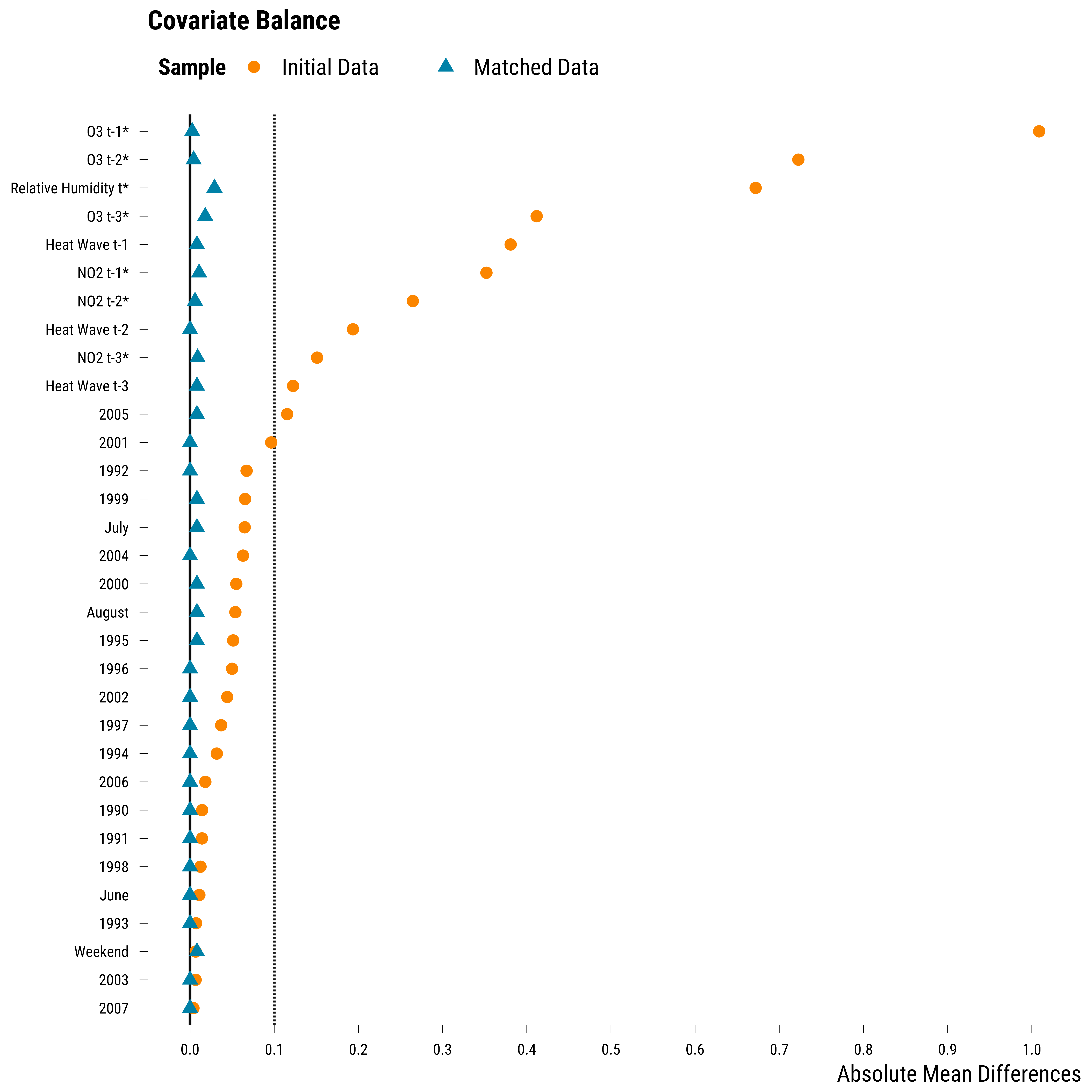
All 122 treated days were matched to control units that satisfy the balancing constraints. We check the evolution of balance after matching:
Please show me the code!
# first we nicely label covariates
cov_labels <- c(
  heat_wave_lag_1 = "Heat Wave t-1",
  heat_wave_lag_2 = "Heat Wave t-2",
  heat_wave_lag_3 = "Heat Wave t-3",
  o3_lag_1 = "O3 t-1",
  o3_lag_2 = "O3 t-2",
  o3_lag_3 = "O3 t-3",
  no2_lag_1 = "NO2 t-1",
  no2_lag_2 = "NO2 t-2",
  no2_lag_3 = "NO2 t-3",
  humidity_relative = "Relative Humidity t",
  weekend = "Weekend",
  month_august = "August",
  month_june = "June",
  month_july = "July",
  year_1990 = "1990",
  year_1991 = "1991",
  year_1992 = "1992",
  year_1993 = "1993",
  year_1994 = "1994",
  year_1995 = "1995",
  year_1996 = "1996",
  year_1997 = "1997",
  year_1998 = "1998",
  year_1999 = "1999",
  year_2000 = "2000",
  year_2001 = "2001",
  year_2002 = "2002",
  year_2003 = "2003",
  year_2004 = "2004",
  year_2005 = "2005",
  year_2006 = "2006",
  year_2007 = "2007"
)

# make the love plot
graph_love_plot_card <- love.plot(
  card_match_1,
  treat = data$heat_wave,
  covs = data_covs,
  abs = TRUE,
  var.order = "unadjusted",
  binary = "raw",
  s.d.denom = "treated",
  thresholds = c(m = .1),
  var.names = cov_labels,
  sample.names = c("Initial Data", "Matched Data"),
  shapes = c("circle", "triangle"),
  colors = c(my_orange, my_blue),
  stars = "std"
) +
  scale_x_continuous(breaks = scales::pretty_breaks(n = 10)) +
  xlab("Absolute Mean Differences") +
  theme_tufte()

# display the graph
graph_love_plot_card
Please show me the code!
# save the graph
ggsave(
  graph_love_plot_card + labs(title = NULL),
  filename = here::here(
    "inputs", "3.outputs",
    "2.graphs",
    "graph_love_plot_card.pdf"
  ),
  width = 20,
  height = 15,
  units = "cm",
  device = cairo_pdf
)
On this graph, we can see that balance has improved a lot after matching. We display below the evolution of the average of standardized mean differences for continuous covariates:
Please show me the code!
| Sample | Average of Standardized Mean Differences | Std. Deviation |
|---|---|---|
| Initial Data | 0.51 | 0.30 |
| Matched Data | 0.01 | 0.01 |
We also display below the evolution of the difference in proportions for binary covariates:
Please show me the code!
| Sample | Average of Proportion Differences | Std. Deviation |
|---|---|---|
| Initial Data | 0.06 | 0.08 |
| Matched Data | 0.00 | 0.00 |
Overall, for both types of covariates, the balance has clearly improved after matching. We save the data on covariates balance in the 3.outputs/1.data/covariates_balance folder.
We retrieve the matched data:
# retrieve matched pairs
data_matched = data[c(t_id_1, c_id_1), ] %>%
  mutate(group_id = card_match_1$group_id)
As for other matching procedure, within and across pairs spillover could be an issue. We display below the distribution of difference in days within pairs:
Please show me the code!
data_matched %>%
  group_by(group_id) %>%
  summarise(difference_days = abs(date[1]-date[2]) %>% as.numeric(.)) %>%
  summarise(
    "Mean" = round(mean(difference_days, na.rm = TRUE), 1),
    "Median" = round(median(difference_days, na.rm = TRUE), 1),
    "Standard Deviation" = round(sd(difference_days, na.rm = TRUE), 1),
    "Minimum" = round(min(difference_days, na.rm = TRUE), 1),
    "Maximum" = round(max(difference_days, na.rm = TRUE), 1)
  ) %>%
  # print the table
  kable(., align = c("l", rep("c", 4)))
| Mean | Median | Standard Deviation | Minimum | Maximum |
|---|---|---|---|---|
| 1828.5 | 1461.5 | 1577.2 | 1 | 5835 |
This table shows that for most pairs, “within” spillovers should not be an issue since the treated day is temporally far away from the control day. In the match dataset, there could however be spillover between pairs. For example, the first lead of a treated day could be used as a control in another pair. We first compute below the minimum of the distance of each treated day with all other control days and then retrieve the proportion of treated days for which the minimum distance with a control unit in another pair is inferior or equal to to 5 days.
Please show me the code!
# retrieve dates of treated units
treated_pairs <- data_matched %>%
  dplyr::select(group_id, heat_wave, date) %>%
  filter(heat_wave == 1)

# retrieve dates of controls
control_pairs <- data_matched %>%
  dplyr::select(group_id, heat_wave, date) %>%
  filter(heat_wave == 0)

# compute proportion for which the distance is inferior or equal to 5 days
distance_5_days <- treated_pairs %>%
  group_by(group_id, date) %>%
  expand(other_date = control_pairs$date) %>%
  filter(date!=other_date) %>%
  mutate(difference = (date-other_date) %>% as.numeric()) %>%
  group_by(group_id) %>%
  filter(difference > 0) %>%
  summarise(min_difference = min(difference)) %>%
  arrange(min_difference) %>%
  summarise(sum(min_difference<=5)/n()*100)
56% of pairs could suffer from a “between” spillover effect.
Re-Matching to Reduce Heterogeneity
Once we have find the largest sample that satisfies the balance constraints, we rematch the pairs according to a covariate that is predictive of YLL: here, we use the June indicator.
# define the matched treatment indicator
t_ind_2 = data$heat_wave[c(t_id_1, c_id_1)]

# re-match according the first lag of o3
dist_mat_2 = abs(outer(data$month_june[t_id_1], data$month_june[c_id_1], "-"))

card_match_2 = distmatch(t_ind_2, dist_mat_2)
  Building the matching problem...
  GLPK optimizer is open...
  Finding the optimal matches...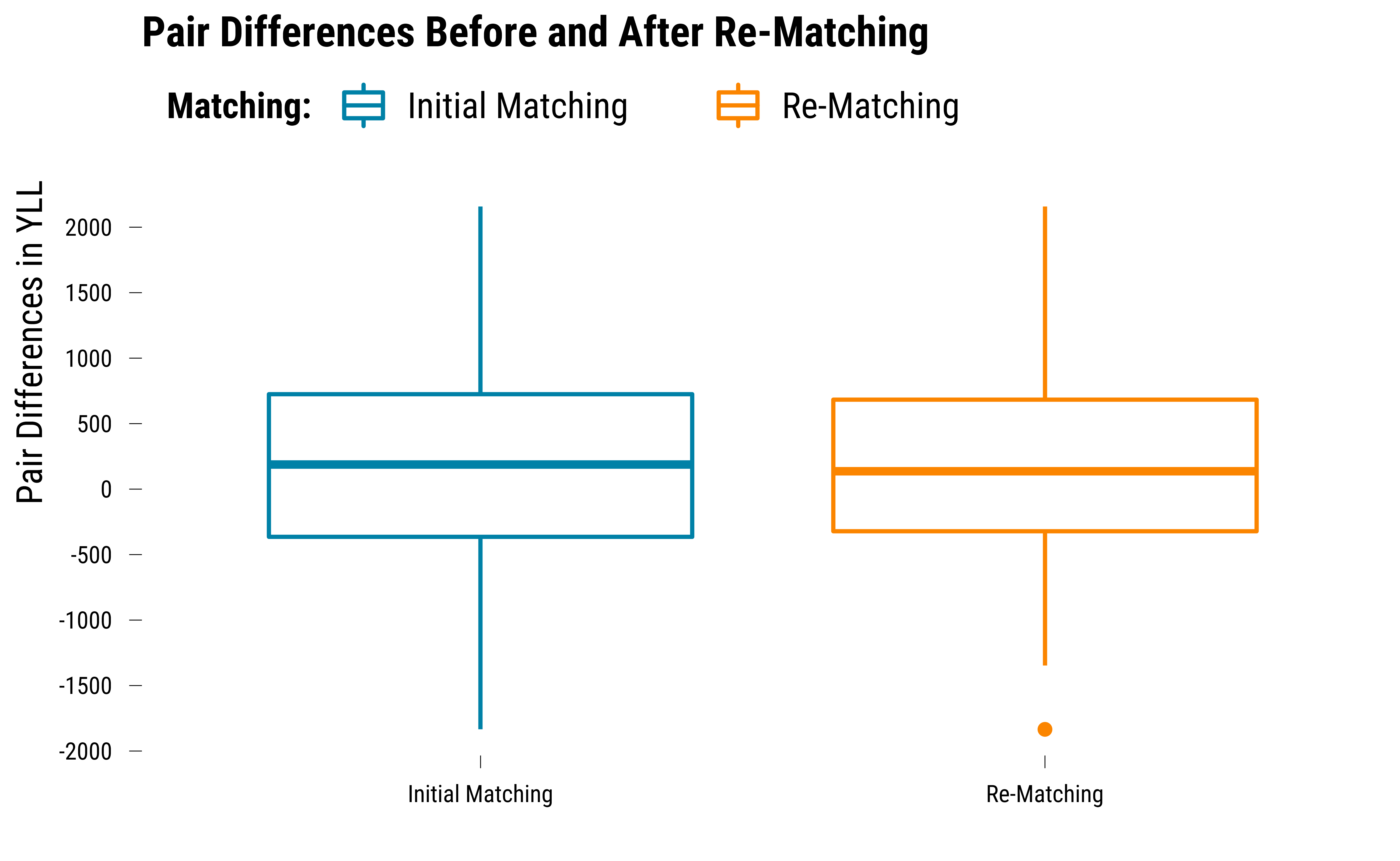
Optimal matches found We check below if the heterogeneity in pair differences has been reduced:
# pair differences in matched data
pair_diff_matched <- data_matched %>%
  dplyr::select(group_id, heat_wave, yll) %>%
  group_by(group_id) %>%
  summarise(yll_diff = yll[1]-yll[2]) %>%
  mutate(matching = "Initial Matching")

# pair differences in rematched data
pair_diff_rematched <- data_rematched %>%
  dplyr::select(group_id, heat_wave, yll) %>%
  group_by(group_id) %>%
  summarise(yll_diff = yll[1]-yll[2]) %>%
  mutate(matching = "Re-Matching")

# boxplot of pair differences
graph_pair_diff_card <- pair_diff_matched %>%
  bind_rows(pair_diff_rematched) %>%
  ggplot(., aes(x = matching, y = yll_diff, colour = matching)) +
  geom_boxplot() +
  scale_color_manual(name = "Matching:", values = c(my_blue, my_orange)) +
  scale_y_continuous(breaks = scales::pretty_breaks(n = 8)) +
  xlab("") + ylab("Pair Differences in YLL") +
  ggtitle("Pair Differences Before and After Re-Matching") +
  theme_tufte()

# display the graph
graph_pair_diff_card
# save the graph
ggsave(
  graph_pair_diff_card + labs(title = NULL),
  filename = here::here("inputs", "3.outputs", "2.graphs", "graph_pair_diff_card.pdf"),
  width = 20,
  height = 15,
  units = "cm",
  device = cairo_pdf
)
The reduction in heterogeinity is very small. The standard deviation of pair differences in YLL was 754 in the first matching and 731 after re-matching.
Analysis of Matched Data
Initial Matched Data
We now move to the analysis of the matched data using a simple regression model where we first regress the YLL on the treatment indicator. We start with the matched data resulting from the initial cardinality matching.
# we fit the regression model
model_match <- lm(yll ~ heat_wave, data = data_matched)

# retrieve the estimate and 95% ci
results_model_match <- tidy(coeftest(
  model_match,
  vcov. = vcovCL,
  cluster = ~ group_id
),
conf.int = TRUE) %>%
  filter(term == "heat_wave") %>%
  dplyr::select(term, estimate, conf.low, conf.high) %>%
  mutate_at(vars(estimate:conf.high), ~ round(., 0))

# display results
results_model_match %>%
  rename(
    "Term" = term,
    "Estimate" = estimate,
    "95% CI Lower Bound" = conf.low,
    "95% CI Upper Bound" = conf.high
  ) %>%
  kable(., align = c("l", "c", "c", "c"))
| Term | Estimate | 95% CI Lower Bound | 95% CI Upper Bound |
|---|---|---|---|
| heat_wave | 194 | 59 | 329 |
We find that the average effect on the treated is equal to +194 years of life lost. The 95% confidence interval is consistent with effects ranging from +59 YLL up to +329 YLL. If we want to increase the precision of our estimate and remove any remaining imbalance in covariates, we can also run a multivariate regression. We adjust below for the same variables used in the cardinality matching:
# we fit the regression model
model_match_w_cov <-
  lm(
    yll ~ heat_wave + heat_wave_lag_1 + heat_wave_lag_2 + heat_wave_lag_3 + o3_lag_1 + o3_lag_2 + o3_lag_3 + no2_lag_1 + no2_lag_2 + no2_lag_3 + humidity_relative + weekend + month + year,
    data = data_matched
  )

# retrieve the estimate and 95% ci
results_model_match_w_cov <- tidy(coeftest(
  model_match_w_cov,
  vcov. = vcovCL,
  cluster = ~ group_id
),
conf.int = TRUE) %>%
  filter(term == "heat_wave") %>%
  dplyr::select(term, estimate, conf.low, conf.high) %>%
  mutate_at(vars(estimate:conf.high), ~ round(., 0))

# display results
results_model_match_w_cov %>%
  rename(
    "Term" = term,
    "Estimate" = estimate,
    "95% CI Lower Bound" = conf.low,
    "95% CI Upper Bound" = conf.high
  ) %>%
  kable(., align = c("l", "c", "c", "c"))
| Term | Estimate | 95% CI Lower Bound | 95% CI Upper Bound |
|---|---|---|---|
| heat_wave | 204 | 77 | 331 |
We find that the average effect on the treated is equal to +204 years of life lost. The 95% confidence interval is consistent with effects ranging from +77 YLL up to +331 YLL. The width of confidence interval is now equal to 254 YLL, which is a bit smaller than the previous interval of 270 YLL.
Re-Matched Data
We then reprocuce the same analysis but for the re-matched data:
# we fit the regression model
model_rematch <- lm(yll ~ heat_wave, data = data_rematched)

# retrieve the estimate and 95% ci
results_model_rematch <- tidy(coeftest(
  model_rematch,
  vcov. = vcovCL,
  cluster = ~ group_id
),
conf.int = TRUE) %>%
  filter(term == "heat_wave") %>%
  dplyr::select(term, estimate, conf.low, conf.high) %>%
  mutate_at(vars(estimate:conf.high), ~ round(., 0))

# display results
results_model_rematch %>%
  rename(
    "Term" = term,
    "Estimate" = estimate,
    "95% CI Lower Bound" = conf.low,
    "95% CI Upper Bound" = conf.high
  ) %>%
  kable(., align = c("l", "c", "c", "c"))
| Term | Estimate | 95% CI Lower Bound | 95% CI Upper Bound |
|---|---|---|---|
| heat_wave | 194 | 64 | 325 |
We find that the average effect on the treated is equal to +194 years of life lost. The 95% confidence interval is consistent with effects ranging from +64 YLL up to +325 YLL. We then run the model where we adjust for covariates:
# we fit the regression model
model_rematch_w_cov <-
  lm(
    yll ~ heat_wave + heat_wave_lag_1 + heat_wave_lag_2 + heat_wave_lag_3 + o3_lag_1 + o3_lag_2 + o3_lag_3 + no2_lag_1 + no2_lag_2 + no2_lag_3 + humidity_relative + weekend + month + year,
    data = data_rematched
  )

# retrieve the estimate and 95% ci
results_model_rematch_w_cov <- tidy(coeftest(
  model_rematch_w_cov,
  vcov. = vcovCL,
  cluster = ~ group_id
),
conf.int = TRUE) %>%
  filter(term == "heat_wave") %>%
  dplyr::select(term, estimate, conf.low, conf.high) %>%
  mutate_at(vars(estimate:conf.high), ~ round(., 0))

# display results
results_model_rematch_w_cov %>%
  rename(
    "Term" = term,
    "Estimate" = estimate,
    "95% CI Lower Bound" = conf.low,
    "95% CI Upper Bound" = conf.high
  ) %>%
  kable(., align = c("l", "c", "c", "c"))
| Term | Estimate | 95% CI Lower Bound | 95% CI Upper Bound |
|---|---|---|---|
| heat_wave | 204 | 77 | 330 |
We find that the average effect on the treated is equal to +204 years of life lost. The 95% confidence interval is consistent with effects ranging from +77 YLL up to +330 YLL. The width of confidence interval is now equal to 253 YLL, which is just a bit smaller than the previous interval of 261 YLL.
Saving Results
We finally save the data on results from propensity score analyses in the 3.outputs/1.data/analysis_results folder.
Please show me the code!
bind_rows(
  results_model_match,
  results_model_match_w_cov,
  results_model_rematch,
  results_model_rematch_w_cov
) %>%
  mutate(
    procedure = c(
      "Cardinality Matching without Covariates Adjustment",
      "Cardinality Matching with Covariates Adjustment",
      "Cardinality Re-Matching without Covariates Adjustment",
      "Cardinality Re-Matching with Covariates Adjustment"
    ),
    sample_size = c(rep(nrow(data_matched), 2), rep(nrow(data_rematched), 2))
  ) %>%
  saveRDS(.,
          here::here(
            "inputs", "3.outputs",
            "1.data",
            "analysis_results",
            "data_analysis_card.RDS"
          ))