In this document, we provide all steps and R codes required to estimate the effect of heat waves of the number of years of life lost (YLL) using propensity score matching. The implementation is done with the fantastic package MatchIt: do not hesitate to explore its very well-made documentation. We also rely on the cobalt package for checking covariate balance.

Should you have any questions, need help to reproduce the analysis or find coding errors, please do not hesitate to contact us at leo.zabrocki@gmail.com.

Required Packages and Data Loading

To reproduce exactly the propensity_score_matching.html document, we first need to have installed:

the R programming language
RStudio, an integrated development environment for R, which will allow you to knit the propensity_score_matching.Rmd file and interact with the R code chunks
the R Markdown package
and the Distill package which provides the template for this document.

Once everything is set up, we load the following packages:

# load required packages
library(knitr) # for creating the R Markdown document
library(here) # for files paths organization
library(tidyverse) # for data manipulation and visualization
library(broom) # for cleaning regression outputs
library(MatchIt) # for matching procedures
library(cobalt) # for assessing covariates balance
library(lmtest) # for modifying regression standard errors
library(sandwich) # for robust and cluster robust standard errors
library(Cairo) # for printing custom police of graphs
library(DT) # for displaying the data as tables

We load our custom ggplot2 theme for graphs:

# load ggplot custom theme
source(here::here("inputs", "2.functions",
                  "script_theme_tufte.R"))
# define nice colors
my_blue <- "#0081a7"
my_orange <- "#fb8500"

We finally load the data:

# load the data
data <-
  readRDS(here::here("inputs", "1.data", "environmental_data.rds")) %>%
  # define year as factors
  mutate(year = as.factor(year))

As a reminder, there are 122 days where an heat wave occurred and 1251 days without heat waves.

Propensity Score Matching

We implement below a propensity score matching procedure where:

each day with an heat wave is matched to the most similar day without heat wave. This is a 1:1 nearest neighbor matching without replacement.
the distance metric used for the matching is the propensity score which is predicted using a logistic model where we regress the heat wave dummy on its three lags, the three lags of ozone and nitrogen dioxide, the relative humidity, the weekend, the month and the year.

We vary the matching distance to see how covariates balance change:

We first match each treated unit to its closest control unit.
We then set the maximum distance to be inferior to 0.5 propensity score standard deviation.

Once treated and control units are matched, we assess whether covariates balance has improved.

We finally estimate the treatment effect.

Matching without a Caliper

We first match each treated unit to its closest control unit using the matchit() function:

# match without caliper
matching_ps_inf_caliper <-
  matchit(
    heat_wave ~ heat_wave_lag_1 + heat_wave_lag_2 + heat_wave_lag_3 +
      humidity_relative + 
      o3_lag_1 + o3_lag_2 + o3_lag_3 +
      no2_lag_1 + no2_lag_2 + no2_lag_3 +
      weekend + month + year,
    data = data
  )

# display summary of the procedure
matching_ps_inf_caliper

A matchit object
 - method: 1:1 nearest neighbor matching without replacement
 - distance: Propensity score
             - estimated with logistic regression
 - number of obs.: 1373 (original), 244 (matched)
 - target estimand: ATT
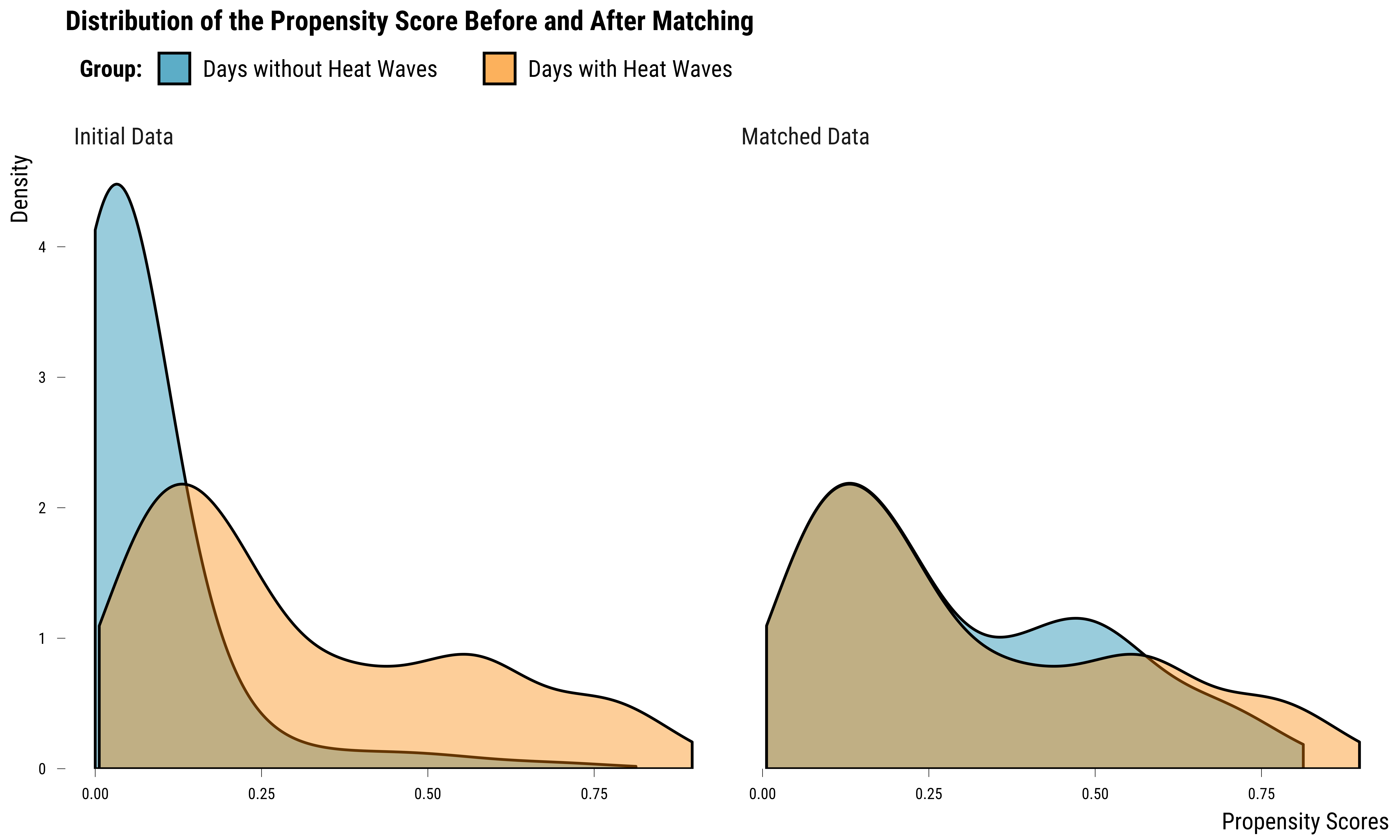
 - covariates: heat_wave_lag_1, heat_wave_lag_2, heat_wave_lag_3, humidity_relative, o3_lag_1, o3_lag_2, o3_lag_3, no2_lag_1, no2_lag_2, no2_lag_3, weekend, month, year

The output of the matching procedure indicates us the method (1:1 nearest neighbor matching without replacement) and the distance (propensity score) we used. It also tells us how many units were matched: 244. We assess how covariates balance has improved by comparing the distribution of propensity scores before and after matching:

Please show me the code!

# distribution of propensity scores
graph_propensity_score_distribution_inf <- bal.plot(
  matching_ps_inf_caliper,
  var.name = "distance",
  which = "both",
  sample.names = c("Initial Data", "Matched Data"),
  type = "density") +
  ggtitle("Distribution of the Propensity Score Before and After Matching") +
  xlab("Propensity Scores") +
  scale_fill_manual(
    name = "Group:",
    values = c(my_blue, my_orange),
    labels = c("Days without Heat Waves", "Days with Heat Waves")
  ) +
  theme_tufte()

# display the graph
graph_propensity_score_distribution_inf

Please show me the code!

# save the graph
ggsave(
  graph_propensity_score_distribution_inf + labs(title = NULL),
  filename = here::here(
    "inputs", "3.outputs",
    "2.graphs",
    "graph_propensity_score_distribution_inf.pdf"
  ),
  width = 16,
  height = 10,
  units = "cm",
  device = cairo_pdf
)

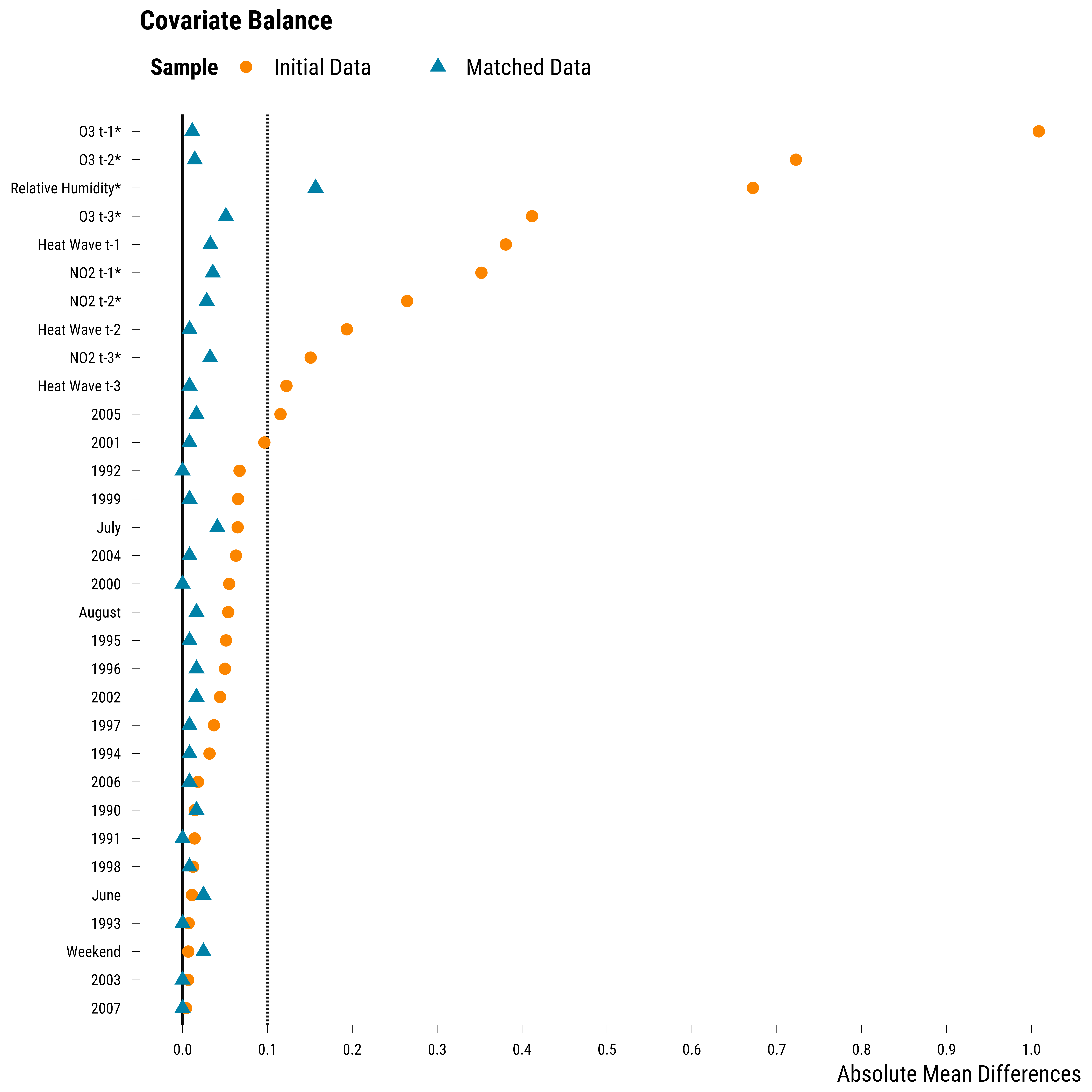
We see on this graph that propensity scores distribution for the two groups better overlap but the two density distributions are still not similar. We can also evaluate the covariates balance using the love.plot() function from the cobalt package and the absolute mean difference as the summary statistic. For binary variables, the absolute difference in proportion is computed. For continuous covariates, denoted with a star, the absolute standardized mean difference is computed (the difference is divided by the standard deviation of the variable for treated units before matching).

Please show me the code!

# first we nicely label covariates
cov_labels <- c(
  heat_wave_lag_1 = "Heat Wave t-1",
  heat_wave_lag_2 = "Heat Wave t-2",
  heat_wave_lag_3 = "Heat Wave t-3",
  o3_lag_1 = "O3 t-1",
  o3_lag_2 = "O3 t-2",
  o3_lag_3 = "O3 t-3",
  no2_lag_1 = "NO2 t-1",
  no2_lag_2 = "NO2 t-2",
  no2_lag_3 = "NO2 t-3",
  humidity_relative = "Relative Humidity",
  weekend = "Weekend",
  month_august = "August",
  month_june = "June",
  month_july = "July",
  year_1990 = "1990",
  year_1991 = "1991",
  year_1992 = "1992",
  year_1993 = "1993",
  year_1994 = "1994",
  year_1995 = "1995",
  year_1996 = "1996",
  year_1997 = "1997",
  year_1998 = "1998",
  year_1999 = "1999",
  year_2000 = "2000",
  year_2001 = "2001",
  year_2002 = "2002",
  year_2003 = "2003",
  year_2004 = "2004",
  year_2005 = "2005",
  year_2006 = "2006",
  year_2007 = "2007"
)

# make the love plot
graph_love_plot_ps_inf <- love.plot(
  matching_ps_inf_caliper,
  drop.distance = TRUE,
  abs = TRUE,
  var.order = "unadjusted",
  binary = "raw",
  s.d.denom = "treated",
  thresholds = c(m = .1),
  var.names = cov_labels,
  sample.names = c("Initial Data", "Matched Data"),
  shapes = c("circle", "triangle"),
  colors = c(my_orange, my_blue),
  stars = "std"
) +
  scale_x_continuous(breaks = scales::pretty_breaks(n = 10)) +
  xlab("Absolute Mean Differences") +
  theme_tufte()

# display the graph
graph_love_plot_ps_inf

Please show me the code!

# save the graph
ggsave(
  graph_love_plot_ps_inf + labs(title = NULL),
  filename = here::here(
    "inputs", "3.outputs",
    "2.graphs",
    "graph_love_plot_ps_inf.pdf"
  ),
  width = 20,
  height = 15,
  units = "cm",
  device = cairo_pdf
)

On this graph, we can see that, for most covariates, balance has improved after matching—yet, for few covariates, the standardized mean difference has increased. We display below the evolution of the average of standardized mean differences for continuous covariates:

Please show me the code!

graph_love_plot_ps_inf[["data"]] %>%
  filter(type == "Contin.") %>%
  group_by(Sample) %>%
  summarise("Average of Standardized Mean Differences" = round(mean(stat), 2),
            "Std. Deviation" = round(sd(stat), 2)) %>%
  kable(align = c("l", "c"))

Sample	Average of Standardized Mean Differences	Std. Deviation
Initial Data	0.51	0.30
Matched Data	0.05	0.05

We also display below the evolution of the difference in proportions for binary covariates:

Please show me the code!

graph_love_plot_ps_inf[["data"]] %>%
  filter(type == "Binary") %>%
  group_by(Sample) %>%
  summarise("Average of Proportion Differences" = round(mean(stat), 2),
            "Std. Deviation" = round(sd(stat), 2)) %>%
  kable(align = c("l", "c"))

Sample	Average of Proportion Differences	Std. Deviation
Initial Data	0.06	0.08
Matched Data	0.01	0.01

Overall, for both types of covariates, the balance has clearly improved after matching.

Matching with a 0.5 Caliper

Until now, we matched each treated unit to its closest control unit according to 1 standard deviation caliper: we could however make sure that a treated unit is not matched to a control unit which is too much different. We do so by setting a caliper of 0.5 standard deviation:

# match without caliper
matching_ps_0.5_caliper <-
  matchit(
    heat_wave ~ heat_wave_lag_1 + heat_wave_lag_2 + heat_wave_lag_3 +
      humidity_relative + 
      o3_lag_1 + o3_lag_2 + o3_lag_3 +
      no2_lag_1 + no2_lag_2 + no2_lag_3 +
      weekend + month + year,
    caliper = 0.5,
    data = data
  )

# display summary of the procedure
matching_ps_0.5_caliper

A matchit object
 - method: 1:1 nearest neighbor matching without replacement
 - distance: Propensity score [caliper]
             - estimated with logistic regression
 - caliper: <distance> (0.073)
 - number of obs.: 1373 (original), 236 (matched)
 - target estimand: ATT
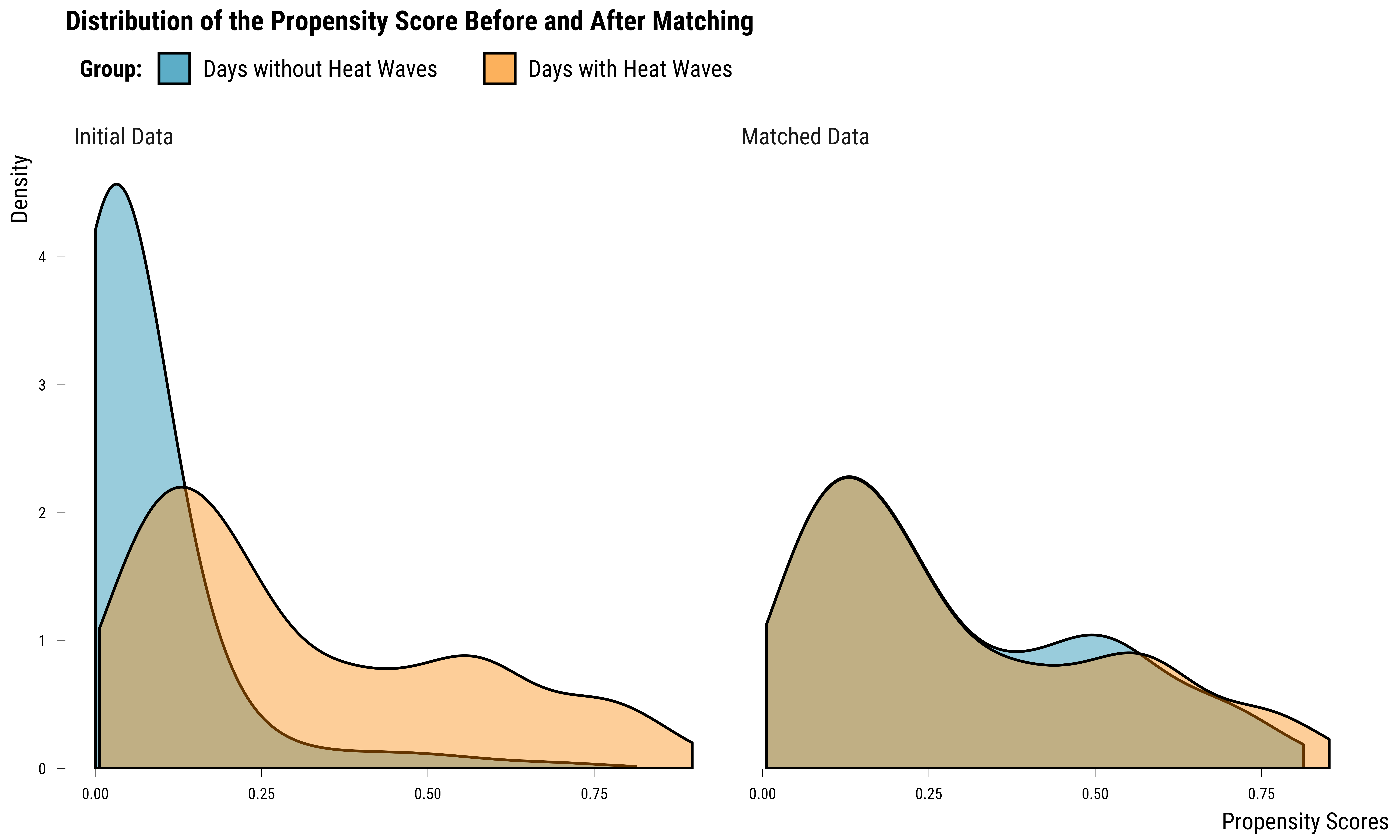
 - covariates: heat_wave_lag_1, heat_wave_lag_2, heat_wave_lag_3, humidity_relative, o3_lag_1, o3_lag_2, o3_lag_3, no2_lag_1, no2_lag_2, no2_lag_3, weekend, month, year

Compared to the matching with an infinite caliper, there are now 236 matched units. We can check whether the propensity score distributions overlap better:

Please show me the code!

# distribution of propensity scores
graph_propensity_score_distribution_0.5 <- bal.plot(
  matching_ps_0.5_caliper,
  var.name = "distance",
  which = "both",
  sample.names = c("Initial Data", "Matched Data"),
  type = "density"
) +
  ggtitle("Distribution of the Propensity Score Before and After Matching") +
  xlab("Propensity Scores") +
  scale_fill_manual(
    name = "Group:",
    values = c(my_blue, my_orange),
    labels = c("Days without Heat Waves", "Days with Heat Waves")
  ) +
  theme_tufte()

# display the graph
graph_propensity_score_distribution_0.5

Please show me the code!

# save the graph
ggsave(
  graph_propensity_score_distribution_0.5 + labs(title = NULL),
  filename = here::here(
    "inputs", "3.outputs",
    "2.graphs",
    "graph_propensity_score_distribution_0.5.pdf"
  ),
  width = 16,
  height = 10,
  units = "cm",
  device = cairo_pdf
)

The overlap seems to be better than the matching without a caliper. We can also evaluate how each covariate balance has improved with a love plot:

Please show me the code!

# make the love plot
graph_love_plot_ps_0.5 <- love.plot(
  heat_wave ~ heat_wave_lag_1 + heat_wave_lag_2 + heat_wave_lag_3 + o3_lag_1 + o3_lag_2 + o3_lag_3  + no2_lag_1 + no2_lag_2 + no2_lag_3 + humidity_relative + weekend + month + year,
  data = data,
  estimand = "ATT",
  weights = list("Without a Caliper" = matching_ps_inf_caliper,
                 "With a 0.5 SD Caliper" = matching_ps_0.5_caliper),
  drop.distance = TRUE,
  abs = TRUE,
  var.order = "unadjusted",
  binary = "raw",
  s.d.denom = "treated",
  thresholds = c(m = .1),
  var.names = cov_labels,
  sample.names = c("Initial Data", "Without a Caliper", "With a 0.5 SD Caliper"),
  shapes = c("circle", "triangle", "square"),
  colors = c(my_orange, my_blue, "#81b29a"),
  stars = "std"
) +
  scale_x_continuous(breaks = scales::pretty_breaks(n = 10)) +
  xlab("Absolute Mean Differences") +
  theme_tufte()

# display the graph
graph_love_plot_ps_0.5

Please show me the code!

# save the graph
ggsave(
  graph_love_plot_ps_0.5,
  filename = here::here(
    "inputs", "3.outputs",
    "2.graphs",
    "graph_love_plot_ps_0.5.pdf"
  ),
  width = 20,
  height = 15,
  units = "cm",
  device = cairo_pdf
)

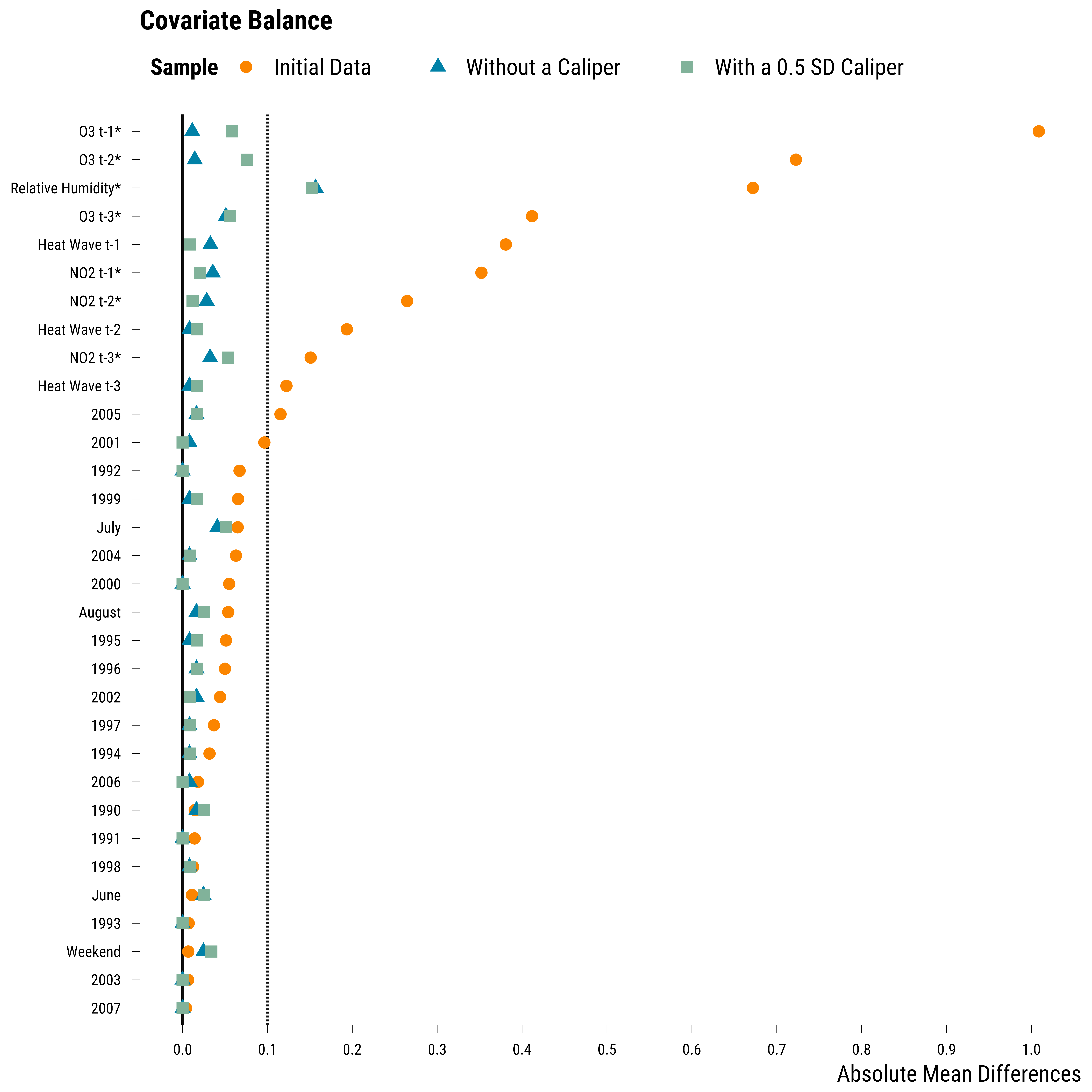
On this graph, it is clear to see that, for several continuous covariates, balance has increased. We display below, for continuous covariates, the average of standardized mean differences for the three datasets:

Please show me the code!

graph_love_plot_ps_0.5[["data"]] %>%
  filter(type == "Contin.") %>%
  group_by(Sample) %>%
  summarise("Average of Standardized Mean Differences" = round(mean(stat), 2),
            "Std. Deviation" = round(sd(stat), 2)) %>%
  kable(align = c("l", "c"))

Sample	Average of Standardized Mean Differences	Std. Deviation
Initial Data	0.51	0.30
Without a Caliper	0.05	0.05
With a 0.5 SD Caliper	0.06	0.05

We also display below the evolution of the difference in proportions for binary covariates:

Please show me the code!

graph_love_plot_ps_0.5[["data"]] %>%
  filter(type == "Binary") %>%
  group_by(Sample) %>%
  summarise("Average of Proportion Differences" = round(mean(stat), 2),
            "Std. Deviation" = round(sd(stat), 2)) %>%
  kable(align = c("l", "c"))

Sample	Average of Proportion Differences	Std. Deviation
Initial Data	0.06	0.08
Without a Caliper	0.01	0.01
With a 0.5 SD Caliper	0.01	0.01

Here, the stricter matching procedure did not help improve the balance of binary covariates.

We finally save the data on covariates balance in the 3.outputs/1.data/covariates_balance folder.

Please show me the code!

graph_love_plot_ps_0.5[["data"]] %>%
  rename_all(tolower) %>%
  mutate(matching_procedure = "Propensity Score Matching") %>%
  dplyr::select(-on.border) %>%
  saveRDS(
    .,
    here::here(
      "inputs", "3.outputs",
      "1.data",
      "covariates_balance",
      "data_cov_balance_ps.RDS"
    )
  )

Analysis of Matched Data

Matched Data without a Caliper

We now move to the analysis of the matched datasets using a simple regression model where we first regress the YLL on the treatment indicator. We start with the matched data resulting from the propensity score without a caliper. We first retrieve the matched dataset:

# we retrieve the matched data
data_ps_inf_caliper <- match.data(matching_ps_inf_caliper)

We then estimate the treatment effect of heat waves with a simple linear regression model:

# we fit the regression model
model_ps_inf_caliper <- lm(yll ~ heat_wave,
                           data = data_ps_inf_caliper,
                           weights = weights)

# retrieve the estimate and 95% ci
results_ps_inf_caliper <- tidy(coeftest(
  model_ps_inf_caliper,
  vcov. = vcovCL,
  cluster = ~ subclass
),
conf.int = TRUE) %>%
  filter(term == "heat_wave") %>%
  dplyr::select(term, estimate, conf.low, conf.high) %>%
  mutate_at(vars(estimate:conf.high), ~ round(., 0))

# display results
results_ps_inf_caliper %>%
  rename(
    "Term" = term,
    "Estimate" = estimate,
    "95% CI Lower Bound" = conf.low,
    "95% CI Upper Bound" = conf.high
  ) %>%
  kable(., align = c("l", "c", "c", "c"))

Term	Estimate	95% CI Lower Bound	95% CI Upper Bound
heat_wave	237	92	383

We find that the average effect on the treated is equal to +237 years of life lost. The 95% confidence interval is consistent with effects ranging from +92 YLL up to +383 YLL. If we want to increase the precision of our estimate and remove any remaining imbalance in covariates, we can also run a multivariate regression. We adjust below for the same variables used in the estimation of the propensity scores:

# we fit the regression model
model_ps_inf_caliper_w_cov <-
  lm(
    yll ~ heat_wave + heat_wave_lag_1 + heat_wave_lag_2 + heat_wave_lag_3 + o3_lag_1 + o3_lag_2 + o3_lag_3 + no2_lag_1 + no2_lag_2 + no2_lag_3 + humidity_relative + weekend + month + year,
    data = data_ps_inf_caliper,
    weights = weights
  )

# retrieve the estimate and 95% ci
results_ps_inf_caliper_w_cov <- tidy(coeftest(
  model_ps_inf_caliper_w_cov,
  vcov. = vcovCL,
  cluster = ~ subclass
),
conf.int = TRUE) %>%
  filter(term == "heat_wave") %>%
  dplyr::select(term, estimate, conf.low, conf.high) %>%
  mutate_at(vars(estimate:conf.high), ~ round(., 0))

# display results
results_ps_inf_caliper_w_cov %>%
  rename(
    "Term" = term,
    "Estimate" = estimate,
    "95% CI Lower Bound" = conf.low,
    "95% CI Upper Bound" = conf.high
  ) %>%
  kable(., align = c("l", "c", "c", "c"))

Term	Estimate	95% CI Lower Bound	95% CI Upper Bound
heat_wave	235	92	378

We find that the average effect on the treated is equal to +235 years of life lost. The 95% confidence interval is consistent with effects ranging from +92 YLL up to +378 YLL. The width of confidence interval is now equal to 286 YLL, which is a bit smaller than the previous interval of 291 YLL.

Matched Data with a 0.5 Caliper

We also estimate the treatment effect for the matched dataset resulting from the matching procedure with a 0.5 caliper. It is very important to note that the target causal estimand is not anymore the the average treatment on the treated as not all treated units could be matched to similar control units: only 118 treated units were matched. We first retrieve the matched dataset:

# we retrieve the matched data
data_ps_0.5_caliper <- match.data(matching_ps_0.5_caliper)

We estimate the treatment effect of heat waves with a simple linear regression model, we get:

# we fit the regression model
model_ps_0.5_caliper <- lm(yll ~ heat_wave,
                          data = data_ps_0.5_caliper,
                          weights = weights)

# retrieve the estimate and 95% ci
results_ps_0.5_caliper <- tidy(coeftest(
  model_ps_0.5_caliper,
  vcov. = vcovCL,
  cluster = ~ subclass
),
conf.int = TRUE) %>%
  filter(term == "heat_wave") %>%
  dplyr::select(term, estimate, conf.low, conf.high) %>%
  mutate_at(vars(estimate:conf.high), ~ round(., 0))

# display results
results_ps_0.5_caliper %>%
  rename(
    "Term" = term,
    "Estimate" = estimate,
    "95% CI Lower Bound" = conf.low,
    "95% CI Upper Bound" = conf.high
  ) %>%
  kable(., align = c("l", "c", "c", "c"))

Term	Estimate	95% CI Lower Bound	95% CI Upper Bound
heat_wave	230	69	390

The estimate is equal to +230 years of life lost. The 95% confidence interval is consistent with effects ranging from +69 YLL up to +390 YLL. We finally run the regression model where we adjust for covariates:

# we fit the regression model
model_ps_0.5_caliper_w_cov <-
  lm(
    yll ~ heat_wave + heat_wave_lag_1 + heat_wave_lag_2 + heat_wave_lag_3 + o3_lag_1 + o3_lag_2 + o3_lag_3 + no2_lag_1 + no2_lag_2 + no2_lag_3 + humidity_relative + weekend + month + year,
    data = data_ps_0.5_caliper,
    weights = weights
  )

# retrieve the estimate and 95% ci
results_ps_0.5_caliper_w_cov <- tidy(coeftest(
  model_ps_0.5_caliper_w_cov,
  vcov. = vcovCL,
  cluster = ~ subclass
),
conf.int = TRUE) %>%
  filter(term == "heat_wave") %>%
  dplyr::select(term, estimate, conf.low, conf.high) %>%
  mutate_at(vars(estimate:conf.high), ~ round(., 0))

# display results
results_ps_0.5_caliper_w_cov %>%
  rename(
    "Term" = term,
    "Estimate" = estimate,
    "95% CI Lower Bound" = conf.low,
    "95% CI Upper Bound" = conf.high
  ) %>%
  kable(., align = c("l", "c", "c", "c"))

Term	Estimate	95% CI Lower Bound	95% CI Upper Bound
heat_wave	241	91	390

We find that the average effect on the treated is equal to +241 years of life lost. The 95% confidence interval is consistent with effects ranging from +91 YLL up to +390 YLL. The width of confidence interval is now equal to 299 YLL, which is just a bit smaller than the previous interval of 321 YLL.

Saving Results

We finally save the data on results from propensity score analyses in the 3.outputs/1.data/analysis_results folder.

Please show me the code!

bind_rows(
  results_ps_inf_caliper,
  results_ps_inf_caliper_w_cov,
  results_ps_0.5_caliper,
  results_ps_0.5_caliper_w_cov
) %>%
  mutate(
    procedure = c(
      "Propensity Score without a Caliper",
      "Propensity Score without a Caliper and with Covariates Adjustment",
      "Propensity Score with a 0.5 SD Caliper",
      "Propensity Score with a 0.5 SD Caliper and with Covariates Adjustment"
    ),
    sample_size = c(rep(sum(
      matching_ps_inf_caliper[["weights"]]
    ), 2), rep(sum(
      matching_ps_0.5_caliper[["weights"]]
    ), 2))
  ) %>%
  saveRDS(.,
          here::here(
            "inputs", "3.outputs",
            "1.data",
            "analysis_results",
            "data_analysis_ps.RDS"
          ))

Propensity Score Matching

Required Packages and Data Loading

Propensity Score Matching

Matching without a Caliper

Matching with a 0.5 Caliper

Analysis of Matched Data

Matched Data without a Caliper

Matched Data with a 0.5 Caliper

Saving Results

Corrections