In this document, we explain why it is very important to check covariates balance and the common support of the data in observational studies. We illustrate these two issues by adapting an example from Jennifer Hill (2011). We simulate a fake dataset on the effects of heat waves on Years of Life Lost (YLL) where covariates are imbalanced and their distribution only partially overlap.

Should you have any questions, need help to reproduce the analysis or find coding errors, please do not hesitate to contact us at leo.zabrocki@gmail.com.

Required Packages and Data Loading

To reproduce exactly the intuition.html document, we first need to have installed:

the R programming language
RStudio, an integrated development environment for R, which will allow you to knit the intuition.Rmd file and interact with the R code chunks
the R Markdown package
and the Distill package which provides the template for this document.

Once everything is set up, we load the following packages:

# load required packages
library(knitr) # for creating the R Markdown document
library(here) # for files paths organization
library(tidyverse) # for data manipulation and visualization
library(broom) # for cleaning regression outputs
library(MatchIt) # for matching procedures
library(Cairo) # for printing custom police of graphs
library(DT) # for building nice table

We load our custom ggplot2 theme for graphs:

# load ggplot custom theme
source(here::here("inputs", "2.functions",
                  "script_theme_tufte.R"))
# define nice colors
my_blue <- "#0081a7"
my_orange <- "#fb8500"

Fake-Data Simulation

Simulation Procedure

We simulate below a fake dataset on the effects of heat waves on Years of Life Lost (YLL):

We create 2000 daily observations.
We assign about 10% of the observations to an heat wave.
We define the distribution of the lag of ozone according to the heat wave status. For days with an heat wave, the lag of ozone is distributed such that N(50, 10\(^2\)). For days without an heat wave, the lag of ozone follows N(20, 10\(^2\)).
For each day, we then create their two potential outcomes Y(0) and Y(1), that is to say their YLL without and with an heat wave. The Y(1) are distributed such that N(1500 + 200 \(\times\) log(O\(_{3_{t-1}}\)), 250\(^2\)). The Y(1) are distributed such that N(2300 + exp(O\(_{3_{t-1}}\) \(\times\) 0.11), 250\(^2\)).
We finally express for each day the observed YLL according the treatment status: YLL = W\(\times\) Y(1) + (1-W)\(\times\) Y(0) where W is the indicator for an heat wave.

Below is the code to simulate the fake-data:

# set seed
set.seed(42)

# set sample size
sample_size <- 2000

data <-
  # create heat wave indicator
  tibble(heat_wave = rbinom(sample_size, size = 1, p = 0.1)) %>%
  rowwise() %>%
  # create ozone lag
  mutate(
    o3_lag = ifelse(heat_wave == 1, rnorm(1, mean = 50, sd = 10), rnorm(1, mean = 20, sd = 10)) %>% abs(.),
    # create potential outcomes
    y_0 = rnorm(1,  1500 + 200 * log(o3_lag), 250),
    y_1 = rnorm(1, 2300 + exp(o3_lag * 0.11), 250),
    # create obsered yll
    y_obs = ifelse(heat_wave == 1, y_1, y_0)
  ) %>%
  ungroup() %>%
  mutate_all(~ round(., 0))

And here are the data:

Please show me the code!

data %>%
    datatable(., options = list(columnDefs = list(
    list(className = 'dt-center', targets = "_all")
  )))

Why Covariates Balance and Common Support Matter

A naive outcome regression analysis may recover a biased estimate of the effect of heat waves on YLL if:

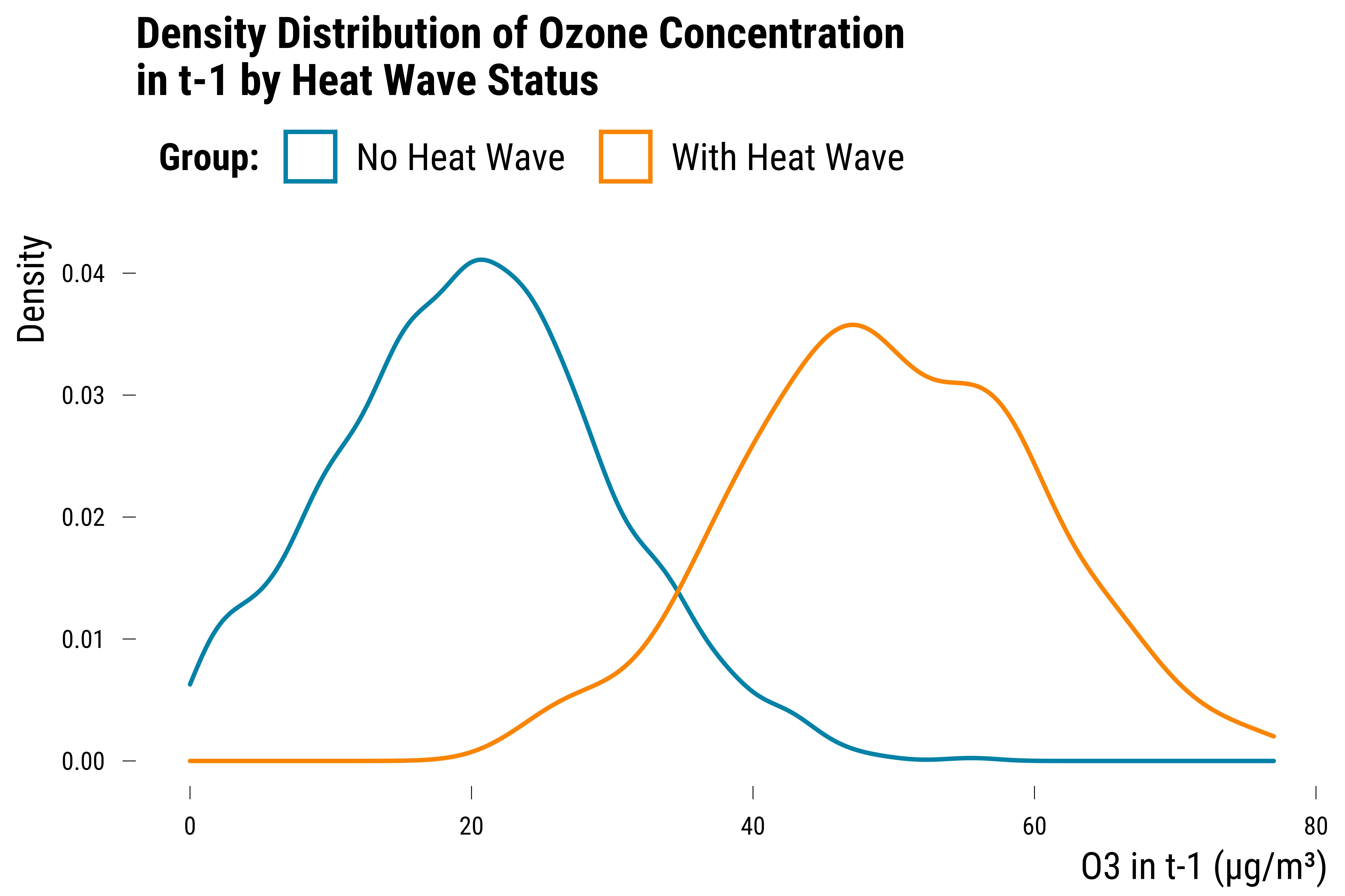
the distributions of confounders are imbalanced, i.e., they are different for days with heat waves compared to days without heat waves. For instance, the lag of ozone concentrations can be on average higher for treated days than control days. This will make the analysis more dependent on the model used to adjust for confounding variables.
the common support of the data is , i.e., there are some treated or c The analysis will be partly based on model extrapolation: if the model is the lag of ozone is balanced across days with and without heat waves:

Please show me the code!

# make the graph
data %>%
  mutate(heat_wave = ifelse(heat_wave==1, "With Heat Wave", "No Heat Wave")) %>%
  ggplot(., aes(x = o3_lag, colour = heat_wave)) +
  geom_density() +
  scale_x_continuous(breaks = scales::pretty_breaks(n = 6)) +
  scale_y_continuous(breaks = scales::pretty_breaks(n = 6)) +
  scale_colour_manual(name = "Group:", values = c(my_blue, my_orange)) +
  labs(x = "O3 in t-1 (µg/m³)", y = "Density", title = "Density Distribution of Ozone Concentration \nin t-1 by Heat Wave Status") +
  theme_tufte()

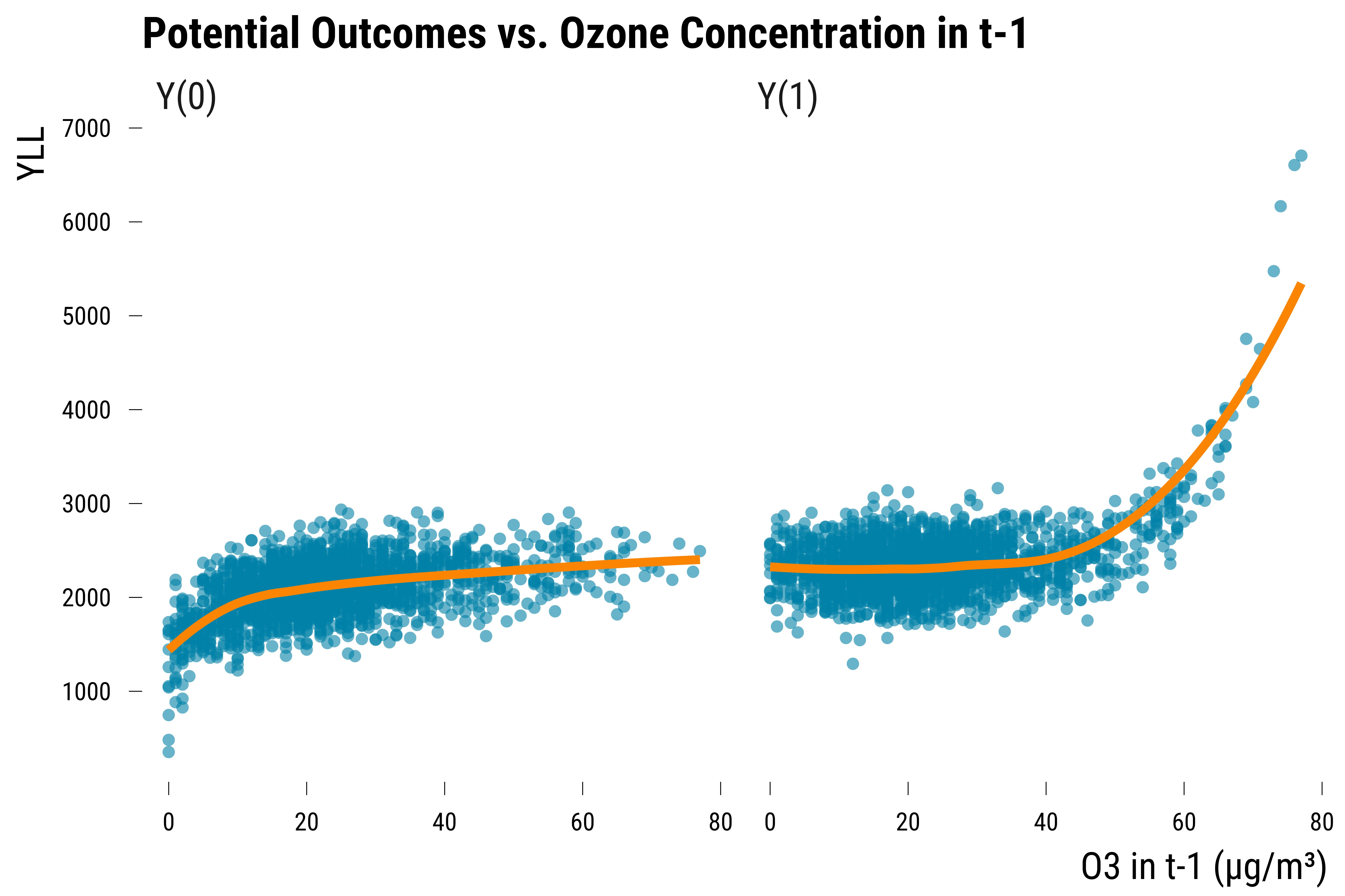
We plot below the potential outcomes against the lag of ozone concentration:

Please show me the code!

# make the graph
graph_po_ozone <- data %>%
  pivot_longer(cols = c(y_0, y_1), names_to = "po", values_to = "value") %>%
  mutate(po = ifelse(po == "y_0", "Y(0)", "Y(1)")) %>%
  ggplot(., aes(x = o3_lag, y = value)) +
  geom_point(shape = 16, colour = my_blue, alpha = 0.6) +
  geom_smooth(method = "loess", se = FALSE, colour = my_orange) +
  scale_x_continuous(breaks = scales::pretty_breaks(n = 6)) +
  scale_y_continuous(breaks = scales::pretty_breaks(n = 6)) +
  facet_wrap(~ po) +
  labs(x = "O3 in t-1 (µg/m³)", y = "YLL", title = "Potential Outcomes vs. Ozone Concentration in t-1") +
  theme_tufte()


# display the graph
graph_po_ozone

Please show me the code!

# save the graph
ggsave(
  graph_po_ozone + labs(title = NULL),
  filename = here::here(
    "inputs", "3.outputs",
    "2.graphs",
    "graph_po_ozone.pdf"
  ),
  width = 18,
  height = 12,
  units = "cm",
  device = cairo_pdf
)

We can see on this graph that the relationship between the lag of ozone and the YLL is non-linear.

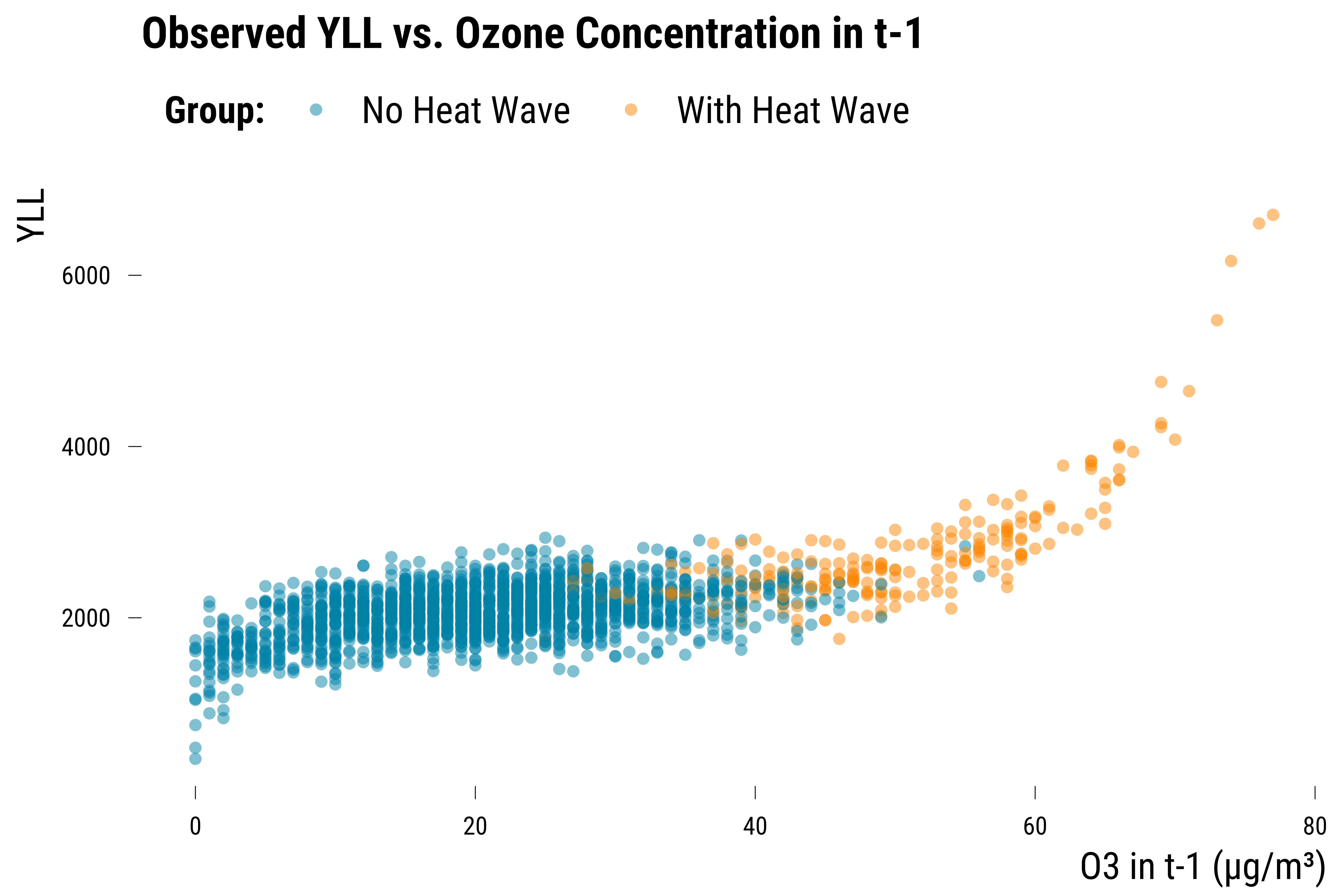
Please show me the code!

data %>%
  mutate(heat_wave = ifelse(heat_wave==1, "With Heat Wave", "No Heat Wave")) %>%
  ggplot(., aes(x = o3_lag, y = y_obs, colour = heat_wave)) +
  geom_point(shape = 16, alpha = 0.5) +
  scale_colour_manual(name = "Group:", values = c(my_blue, my_orange)) +
  
  labs(x = "O3 in t-1 (µg/m³)", y = "YLL", title = "Observed YLL vs. Ozone Concentration in t-1") +
  theme_tufte()

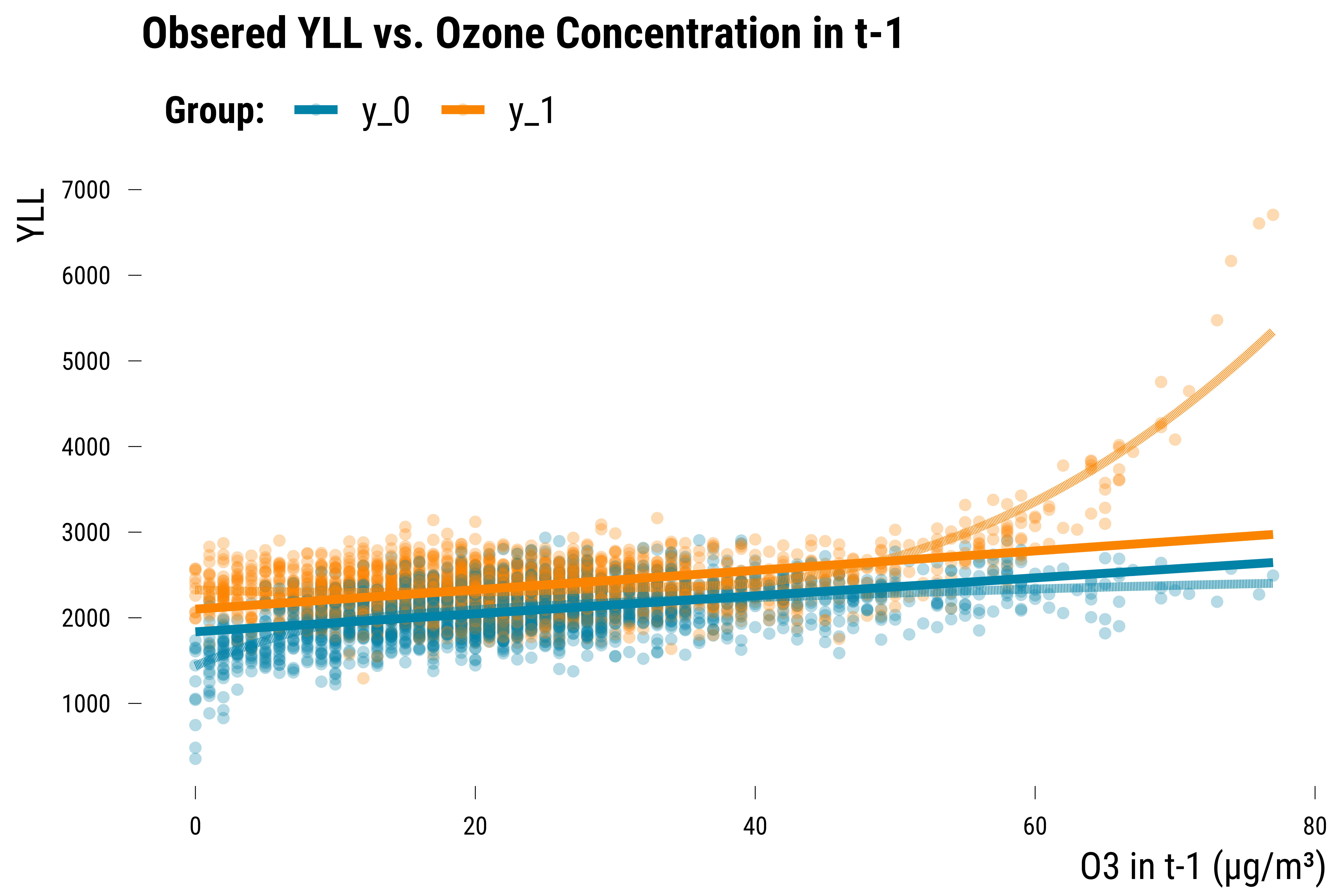
Please show me the code!

data %>%
  pivot_longer(cols = c(y_0, y_1), names_to = "potential_outcome", values_to = "value") %>%
  ggplot(., aes(x = o3_lag, y = value, colour = potential_outcome)) +
  geom_point(shape = 16, alpha = 0.3) +
  geom_smooth(method = "lm", se = FALSE) +
  geom_smooth(method = "loess", se = FALSE, linetype = "dashed") +
  scale_x_continuous(breaks = scales::pretty_breaks(n = 6)) +
  scale_y_continuous(breaks = scales::pretty_breaks(n = 6)) +
  scale_colour_manual(name = "Group:", values = c(my_blue, my_orange)) +
  labs(x = "O3 in t-1 (µg/m³)", y = "YLL", title = "Obsered YLL vs. Ozone Concentration in t-1") +
  theme_tufte()

Values of Causal Estimands

We can finally compute the values of the causal effects of heat waves for:

the days impacted by heat waves. This causal estimand is called the Average Treatment effect on the Treated (ATT).
the days not impacted by heat waves. This causal estimand is called the Average Treatment effect on the Controls (ATC).
all days. This causal estimand is called the Average Treatment Effect (ATE).

# compute att
att <- data %>%
  filter(heat_wave==1) %>%
  summarise(att = mean(y_1-y_0)) %>%
  as_vector()

# compute atc
atc <- data %>%
  filter(heat_wave==0) %>%
  summarise(atc = mean(y_1-y_0)) %>%
  as_vector()

# compute ate
ate <- data %>%
  summarise(ate = mean(y_1-y_0)) %>%
  as_vector()

We display below the values of the three causal estimands:

Please show me the code!

# display results
tibble("ATT" = att, "ATC" = atc, "ATE" = ate) %>%
  mutate_all(~ round(., 0)) %>%
  kable(., align = c("c", "c", "c"))

ATT	ATC	ATE
466	262	284

The ATT is equal to +466 YLL.
The ATC is equal to +262 YLL.
The ATE is equal to +284 YLL.

Analysis of Simulated Data

In this section, we try to estimate the causal effect on heat waves on YLL. The advantage of having simulated the data is that we know the true value of the causal estimands.

Fist, we proceed with an outcome regression approach. In a first model, we simply regress the observed YLL on the dummy for the occurrence of an heat wave:

Please show me the code!

lm(y_obs ~ heat_wave + o3_lag, data = data) %>%
  tidy(., conf.int = TRUE) %>%
  filter(term == "heat_wave") %>%
  dplyr::select(term, estimate, conf.low, conf.high) %>%
  mutate_at(vars(estimate:conf.high), ~ round(., 0)) %>%
  rename(
    "Term" = term,
    "Estimate" = estimate,
    "95% CI Lower Bound" = conf.low,
    "95% CI Upper Bound" = conf.high
  ) %>%
  kable(., align = c("l", "c", "c", "c"))

Term	Estimate	95% CI Lower Bound	95% CI Upper Bound
heat_wave	149	88	211

This outcome regression approach does not recover the value of any of the causal estimands. We could also try to fit a second model where we include a quadric term of the lag of ozone:

Please show me the code!

lm(y_obs ~ heat_wave + o3_lag + I(o3_lag^2), data = data) %>%
  tidy(., conf.int = TRUE) %>%
  filter(term == "heat_wave") %>%
  dplyr::select(term, estimate, conf.low, conf.high) %>%
  mutate_at(vars(estimate:conf.high), ~ round(., 0)) %>%
  rename(
    "Term" = term,
    "Estimate" = estimate,
    "95% CI Lower Bound" = conf.low,
    "95% CI Upper Bound" = conf.high
  ) %>%
  kable(., align = c("l", "c", "c", "c"))

Term	Estimate	95% CI Lower Bound	95% CI Upper Bound
heat_wave	-97	-167	-28

The estimate is now negative! When the data are imbalanced and there is a lack of overlap in covariates, the analysis can be very sensitivity to the model.

Instead of directly estimating a regression model, we could first prune the data to only keep the control units with similar ozone concentrations. To do so, we implement a propensity score matching procedure where:

each day with an heat wave is matched to the most similar day without heat wave. This is a 1:1 nearest neighbor matching without replacement.
the distance metric used for the matching is the propensity score which is predicted using a logistic model where we regress the heat wave dummy on the lag of ozone. Here, we set the maximum distance to be inferior to 0.1 propensity score standard deviation.

We implement the matching with the following code:

# match with a 0.1 caliper
matching_ps <-
  matchit(
    heat_wave ~ o3_lag,
    caliper = 0.1,
    data = data
  )

# display summary of the procedure
matching_ps

A matchit object
 - method: 1:1 nearest neighbor matching without replacement
 - distance: Propensity score [caliper]
             - estimated with logistic regression
 - caliper: <distance> (0.026)
 - number of obs.: 2000 (original), 154 (matched)
 - target estimand: ATT
 - covariates: o3_lag

We can see that 77 days with an heat wave could be matched to a similar day without an heat wave. It is here important to note that the causal estimand that is target by the matching result is no longer the ATT since only 77 treated days were matched. In the initial sample, there were 215 days with an heat wave. Given the value of the caliper we set, a large fraction of treated units do not have any empirical counterfactuals.

We then check whether covariates balance has increased. Before the matching, the distribution of the propensity score and the lag of ozone was imbalanced:

# summary of balance before matching
summary(matching_ps)[["sum.all"]][1:2, 1:3]

         Means Treated Means Control Std. Mean Diff.
distance     0.7301413    0.03250399        2.197374
o3_lag      49.6232558   20.18095238        2.788063

After the matching, the balance has improved:

# summary of balance after matching
summary(matching_ps)[["sum.matched"]][1:2, 1:3]

         Means Treated Means Control Std. Mean Diff.
distance     0.3734448     0.3728867     0.001757969
o3_lag      39.6363636    39.0909091     0.051652272

We finally estimate the causal of heat waves on YLL for the matched units. As we simulated the data, we can first compute the true value of heat waves on YLL:

# we retrieve the matched data
data_ps <- match.data(matching_ps)

# compute the true effect for the matched data
true_effect_matching  <- data_ps %>%
  filter(heat_wave==1) %>%
  summarise(att = round(mean(y_1-y_0), 0)) %>%
  as_vector()

The true value of the causal effect of heat waves is equal to +234 YLL. We simply estimate this effect by regressing the observed YLL on the dummy for the occurrence of an heat wave:

Please show me the code!

lm(y_obs ~ heat_wave + o3_lag, data = data_ps) %>%
  tidy(., conf.int = TRUE) %>%
  filter(term == "heat_wave") %>%
  dplyr::select(term, estimate, conf.low, conf.high) %>%
  mutate_at(vars(estimate:conf.high), ~ round(., 0)) %>%
  rename(
    "Term" = term,
    "Estimate" = estimate,
    "95% CI Lower Bound" = conf.low,
    "95% CI Upper Bound" = conf.high
  ) %>%
  kable(., align = c("l", "c", "c", "c"))

Term	Estimate	95% CI Lower Bound	95% CI Upper Bound
heat_wave	231	91	371

Our estimate is nearly equal to the true value of the causal effect! However, it is important to note that if we add a quadratic term for the lag og ozone, our estimate moves away from the true value of the causal effect:

Please show me the code!

lm(y_obs ~ heat_wave + o3_lag + I(o3_lag^2), data = data_ps) %>%
  tidy(., conf.int = TRUE) %>%
  filter(term == "heat_wave") %>%
  dplyr::select(term, estimate, conf.low, conf.high) %>%
  mutate_at(vars(estimate:conf.high), ~ round(., 0)) %>%
  rename(
    "Term" = term,
    "Estimate" = estimate,
    "95% CI Lower Bound" = conf.low,
    "95% CI Upper Bound" = conf.high
  ) %>%
  kable(., align = c("l", "c", "c", "c"))

Term	Estimate	95% CI Lower Bound	95% CI Upper Bound
heat_wave	176	85	267

Matching is not a panacea but should reduce model-dependence compared to an outcome regression approach.

Intuition for the Importance of Covariates Balance and Common Support

Required Packages and Data Loading

Fake-Data Simulation

Simulation Procedure

Why Covariates Balance and Common Support Matter

Values of Causal Estimands

Analysis of Simulated Data

Corrections