In this document, we display the results of the three matching procedures we implemented.

Should you have any questions, need help to reproduce the analysis or find coding errors, please do not hesitate to contact us at leo.zabrocki@gmail.com.

Required Packages and Data Loading

To reproduce exactly the summary_results.html document, we first need to have installed:

the R programming language
RStudio, an integrated development environment for R, which will allow you to knit the summary_results.Rmd file and interact with the R code chunks
the R Markdown package
and the Distill package which provides the template for this document.

Once everything is set up, we load the following packages:

# load required packages
library(knitr) # for creating the R Markdown document
library(here) # for files paths organization
library(tidyverse) # for data manipulation and visualization
library(Cairo) # for printing custom police of graphs

We load our custom ggplot2 theme for graphs:

# load ggplot custom theme
source(here::here("inputs", "2.functions",
                  "script_theme_tufte.R"))
# define nice colors
my_blue <- "#0081a7"
my_orange <- "#fb8500"

Covariates Balance Results

We load and clean the data on covariates balance for each matching procedure:

# load and bind data
files <- dir(
  path = here::here("inputs",
                    "3.outputs",
                    "1.data",
                    "covariates_balance"),
  pattern = "*.RDS",
  full.names = TRUE
)

data_cov_balance <- files %>%
  map( ~ readRDS(.)) %>%
  reduce(rbind)

# recode type
data_cov_balance <- data_cov_balance %>%
  mutate(
    type = case_when(
      type == "Binary" ~ "Binary",
      type == "Contin." ~ "Continuous",
      type == "binary" ~ "Binary",
      type == "continuous" ~ "Continuous"
    )
  )

# clean data for summary statistics
data_cm_card <- data_cov_balance %>%
  filter(matching_procedure %in% c("Coarsened Exact Matching", "Cardinality Matching")) %>%
  filter(sample == "Matched Data") %>%
  dplyr::select(var, type, stat, matching_procedure)

data_initial <- data_cov_balance %>%
  filter(matching_procedure == "Coarsened Exact Matching" & sample == "Initial Data") %>%
  dplyr::select(-matching_procedure) %>%
  rename(matching_procedure = sample)

data_ps <- data_cov_balance %>%
  filter(sample %in% c("Without a Caliper", "With a 0.5 SD Caliper")) %>%
  mutate(
    matching_procedure = ifelse(
      sample == "Without a Caliper",
      "Propensity Score Matching without a Caliper",
      "Propensity Score Matching with a 0.5 SD Caliper"
    )) %>%
  dplyr::select(-sample)

# bind clean data
data_cov_balance <- bind_rows(data_initial, data_ps) %>%
  bind_rows(., data_cm_card)

We compute summary statistics on balance for continuous variables:

Matching Procedure	Average of Standardized Mean Differences	Std. Deviation
Initial Data	0.51	0.30
Propensity Score Matching without a Caliper	0.05	0.05
Propensity Score Matching with a 0.5 SD Caliper	0.06	0.05
Coarsened Exact Matching	0.04	0.03
Cardinality Matching	0.01	0.01

We can see that cardinality matching is the most effective procedure to reduce imbalance for continuous covariates.

We compute summary statistics on balance for binary variables:

Matching Procedure	Average of Proportion Differences	Std. Deviation
Initial Data	0.06	0.08
Propensity Score Matching without a Caliper	0.01	0.01
Propensity Score Matching with a 0.5 SD Caliper	0.01	0.01
Coarsened Exact Matching	0.03	0.03
Cardinality Matching	0.00	0.00

Similarly, cardinality matching is also the most effective procedure to reduce imbalance for discrete covariates.

Analysis Results

We load the results on the estimates of treatment effect sizes for the matching procedures and the regression outcome approach:

# load and bind data
files <- dir(
  path = here::here("inputs",
                    "3.outputs",
                    "1.data",
                    "analysis_results"),
  pattern = "*.RDS",
  full.names = TRUE
)

data_analysis_results <- files %>%
  map(~ readRDS(.)) %>% 
  reduce(rbind)

We display below the summary of results in a table:

Procedure	Sample Size	Estimate	95% CI	Width of CI
Outcome Regression Model without Covariates Adjustment	1373	388	(297; 479)	182
Outcome Regression Model with Covariates Adjustment	1373	240	(143; 337)	194
Propensity Score without a Caliper	244	237	(92; 383)	291
Propensity Score without a Caliper and with Covariates Adjustment	244	235	(92; 378)	286
Propensity Score with a 0.5 SD Caliper	236	230	(69; 390)	321
Propensity Score with a 0.5 SD Caliper and with Covariates Adjustment	236	241	(91; 390)	299
Coarsened Matching without Covariates Adjustment	158	221	(71; 370)	299
Coarsened Matching with Covariates Adjustment	158	308	(165; 450)	285
Cardinality Matching without Covariates Adjustment	244	194	(59; 329)	270
Cardinality Matching with Covariates Adjustment	244	204	(77; 331)	254
Cardinality Re-Matching without Covariates Adjustment	244	194	(64; 325)	261
Cardinality Re-Matching with Covariates Adjustment	244	204	(77; 330)	253

We display below the summary of results in a graph:

Please show me the code!

# add column for stripes
data_analysis_results <- data_analysis_results %>%
  mutate(group_index = rep(1:6, each = 2), 
         stripe = ifelse((group_index %% 2) == 0, "Grey", "White"))

# make the graph
graph_results_ci <-
  data_analysis_results %>%
  mutate(
    procedure = fct_relevel(
      procedure,
      "Outcome Regression Model without Covariates Adjustment",
      "Outcome Regression Model with Covariates Adjustment",
      "Propensity Score without a Caliper",
      "Propensity Score without a Caliper and with Covariates Adjustment",
      "Propensity Score with a 0.5 SD Caliper",
      "Propensity Score with a 0.5 SD Caliper and with Covariates Adjustment",
      "Coarsened Matching without Covariates Adjustment",
      "Coarsened Matching with Covariates Adjustment",
      "Cardinality Matching without Covariates Adjustment",
      "Cardinality Matching with Covariates Adjustment",
      "Cardinality Re-Matching without Covariates Adjustment",
      "Cardinality Re-Matching with Covariates Adjustment"
    )
  ) %>%
  ggplot(.,
         aes(
           x = estimate,
           y = fct_rev(procedure),
         )) +
    geom_rect(
    aes(fill = stripe),
    ymin = as.numeric(as.factor(data_analysis_results$procedure))-0.495,
    ymax = as.numeric(as.factor(data_analysis_results$procedure))+0.495,
    xmin = -Inf,
    xmax = Inf,
    color = NA,
    alpha = 0.4
  ) +
  geom_vline(xintercept = 0) +
  geom_pointrange(aes(xmin = conf.low, xmax = conf.high), size = 0.5, colour = my_blue, lwd = 0.8) +
  scale_x_continuous(breaks = scales::pretty_breaks(n = 10)) +
  scale_fill_manual(values = c('gray86', "white")) +
  guides(fill = FALSE) +
  ylab("") + xlab("Estimates for Heat Wave Effects on YLL") +
  theme_tufte() +
  theme(axis.ticks.y = element_blank())


# print the graph
graph_results_ci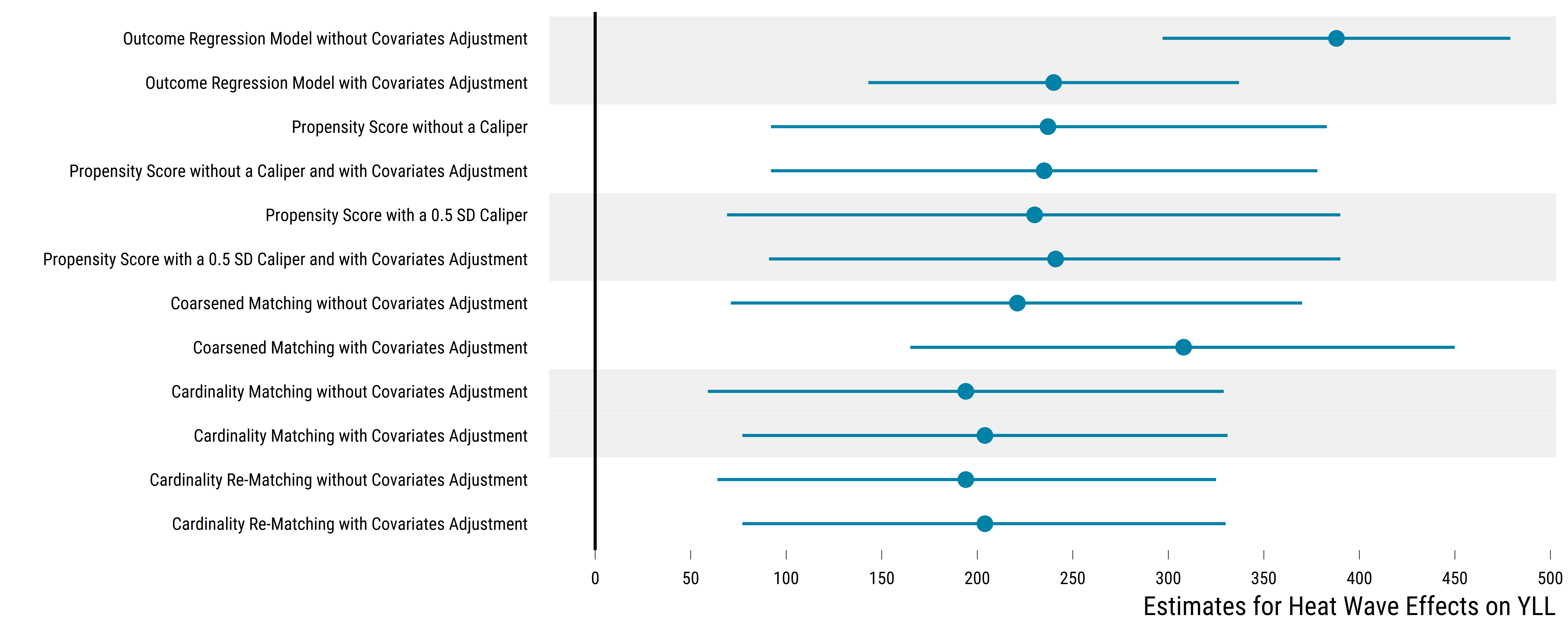

Please show me the code!

# save the graph
ggsave(
  graph_results_ci,
  filename = here::here(
    "inputs",
    "3.outputs",
    "2.graphs",
    "graph_results_ci.pdf"
  ),
  width = 25,
  height = 12,
  units = "cm",
  device = cairo_pdf
)

Overall, all matching procedures lead to less precise estimates than the outcome regression model with covariates adjustment: the width of matching 95% confidence interval ranges from 253 YLL (for cardinality re-matching with covariates adjustment) up to 306 YLL (for propensity score matching with a 0.5 SD caliper). Matching point estimates are relatively similar to the point estimate of +239 YLL found with an outcome regression model with covariates adjustment: matching point estimates vary from +194 YLL (for cardinality matching without covariates adjustment) up to +297 YLL (for coarsened matching with covariates adjustment). Of course, we directly cannot compare the values of point estimates as each rely on a different sample.

Summary of Results

Required Packages and Data Loading

Covariates Balance Results

Analysis Results

Corrections