In this document, we provide all steps and R codes required to analyse the effect of heat waves on the number of years of life lost (YLL ) using an outcome regression approach. This is often the standard procedure followed by researchers in environmental epidemiology: covariates balance is not discussed and confounding variables are adjusted for with a multivariate regression model.
Should you have any questions, need help to reproduce the analysis or find coding errors, please do not hesitate to contact us at leo.zabrocki@gmail.com.
Required Packages
To reproduce exactly the outcome_regression_analysis.html document, we first need to have installed:
- the R programming language
- RStudio, an integrated development environment for R, which will allow you to knit the outcome_regression_analysis.Rmd file and interact with the R code chunks
- the R Markdown package
- and the Distill package which provides the template for this document.
Once everything is set up, we load the following packages:
# load required packages
library(knitr) # for creating the R Markdown document
library(here) # for files paths organization
library(tidyverse) # for data manipulation and visualization
library(broom) # for cleaning regression outputs
library(Cairo) # for printing custom police of graphs
library(DT) # for displaying the data as tables
We finally load our custom ggplot2 theme for graphs:
Regression Analysis
We load the simulated environmental data:
Graphical Difference in YLL
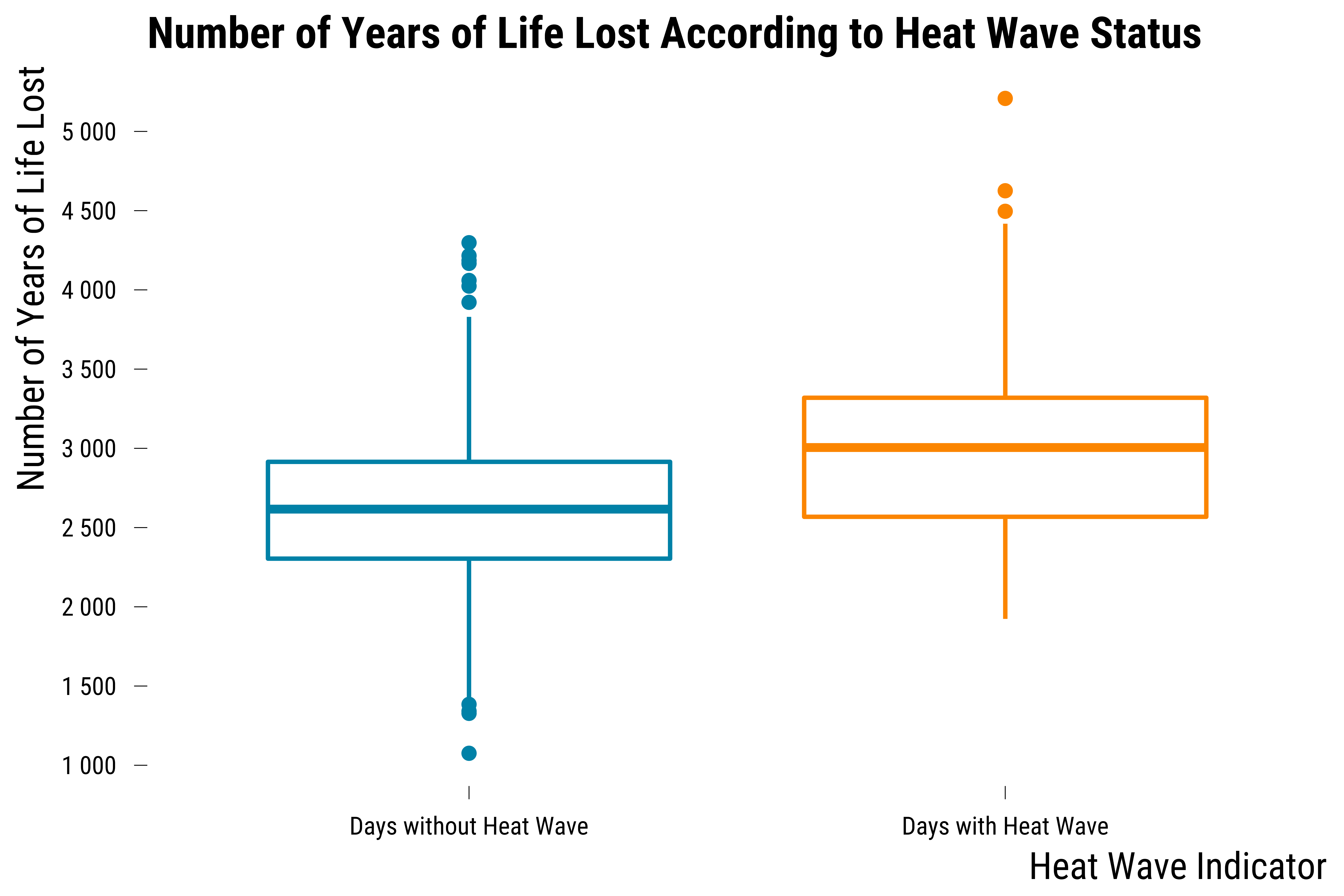
To explore whether heat waves lead to an increase in YLL , we could first compare the distribution of the outcome between days with heat waves and days without heat waves:
Please show me the code!
# make graph
graph_boxplot_YLL  <- data %>%
  # recode heat_wave variable
  mutate(heat_wave = ifelse(heat_wave == 1, "Days with Heat Wave", "Days without Heat Wave")) %>%
  # make a boxplots graph
  ggplot(., aes(
    x = fct_rev(heat_wave),
    y = yll,
    color = fct_rev(heat_wave)
  )) +
  geom_boxplot() +
  scale_color_manual(values = c(my_blue, my_orange)) +
  scale_y_continuous(
    breaks = scales::pretty_breaks(n = 8),
    labels = function(x)
      format(x, big.mark = " ", scientific = FALSE)
  ) +
  xlab("Heat Wave Indicator") +
  ylab("Number of Years of Life Lost") +
  ggtitle("Number of Years of Life Lost According to Heat Wave Status") +
  theme_tufte() +
  guides(color = FALSE)

# display the graph
graph_boxplot_YLL
Please show me the code!
# save the graph
ggsave(
  graph_boxplot_YLL + labs(title = NULL),
  filename = here::here("inputs", "3.outputs", "2.graphs", "graph_boxplot_YLL .pdf"),
  width = 10,
  height = 10,
  units = "cm",
  device = cairo_pdf
)
On this graph, we can see that the median of the number of years of life lost for days with heat waves is higher by 390 YLL than the median of days without heat waves.
Crude Regression Analysis
We then regress the observed number of years of life lost
(y_obs) on the indicator for the occurrence of a heat wave
(heat_wave) to get a crude estimate of the difference:
\(\text{YLL }_{t} = \alpha + \beta\text{HW}_{t} + \epsilon_{t}\)
where \(t\) is the time index, \(\beta\) is the coefficient of interest and \(\epsilon\) the error term. We implement this model in R with the following code:
# run the model and clean output
output_crude_regression <- data %>%
  lm(yll ~ heat_wave, data = .) %>%
  tidy(., conf.int = TRUE) %>%
  filter(term == "heat_wave") %>%
  dplyr::select(term, estimate, conf.low, conf.high) %>%
  mutate_at(vars(estimate:conf.high), ~ round(., 0))

# display output
output_crude_regression %>%
  rename(
    "Term" = term,
    "Estimate" = estimate,
    "95% CI Lower Bound" = conf.low,
    "95% CI Upper Bound" = conf.high
  ) %>%
  kable(., align = c("l", "c", "c", "c"))
| Term | Estimate | 95% CI Lower Bound | 95% CI Upper Bound |
|---|---|---|---|
| heat_wave | 388 | 297 | 479 |
The estimate for the effect of heat waves on YLL is equal to + 388 and the data are consistent with effects ranging from 297 up to 479.
Regression Analysis with Adjustment for Confounders
We finally run a regression where we adjust for potential confounders such as calendar variables (i.e., the month, the year and their interaction), weather parameters (i.e., the relative humidity) and lags of air pollutants (i.e., NO\(_{2}\) and O\(_{3}\)). We also include variables such as the weekend as it is good predictor of the outcome. This regression model can be written such that:
\(\text{YLL }_{t} = \alpha + \beta\text{HW}_{t} + \theta\text{Hum}_{t} + \textbf{P}_{t-1:t-3}\phi + \textbf{C}_{t}\gamma + \epsilon_{t}\)
where \(Hum\) is the relative humidity, \(P\) the vector of air pollutants variables and \(C_{t}\) the vector of calendar indicators. We implement this model in R with the following code:
# run the model and clean ouput
output_adjusted_regression <- data %>%
  lm(yll ~ heat_wave + heat_wave_lag_1 + heat_wave_lag_2 + heat_wave_lag_3 +
       humidity_relative +
       o3_lag_1 + o3_lag_2 + o3_lag_3 +
       no2_lag_1 + no2_lag_2 + no2_lag_3 +
       weekend + month*as.factor(year),
     data = .) %>%
  tidy(., conf.int = TRUE) %>%
  filter(term == "heat_wave") %>%
  dplyr::select(term, estimate, conf.low, conf.high) %>%
  mutate_at(vars(estimate:conf.high), ~ round(., 0))

# display output
output_adjusted_regression %>%
  rename(
    "Term" = term,
    "Estimate" = estimate,
    "95% CI Lower Bound" = conf.low,
    "95% CI Upper Bound" = conf.high
  ) %>%
  kable(., align = c("l", "c", "c", "c"))
| Term | Estimate | 95% CI Lower Bound | 95% CI Upper Bound |
|---|---|---|---|
| heat_wave | 240 | 143 | 337 |
The estimate for the effect of heat waves on YLL is equal to + 240 and the data are consistent with effects ranging from 143 up to 337. This regression model may be too simple. We could include other lags of the variables and use a cubic spline function to better model variations in YLL.
We finally save the results from the two outcome regression models in
the 3.outputs/1.data/analysis_results folder:
bind_rows(output_crude_regression,
  output_adjusted_regression) %>%
  mutate(
    procedure = c(
      "Outcome Regression Model without Covariates Adjustment",
      "Outcome Regression Model with Covariates Adjustment"
    ),
    sample_size = nrow(data)) %>%
  saveRDS(
    .,
    here::here(
      "inputs",
      "3.outputs",
      "1.data",
      "analysis_results",
      "data_analysis_regression.RDS"
    )
  )