In this document, we take great care providing all steps and R codes required to analyze the effects of entering cruise traffic on air pollutants. We compare hours where:

treated units are hours with positive entering cruise traffic in t.
control units are hours without entering cruise traffic in t.

We adjust for calendar calendar indicator and weather confounding factors.

Should you have any questions, need help to reproduce the analysis or find coding errors, please do not hesitate to contact us at leo.zabrocki@gmail.com and marion.leroutier@hhs.se.

Required Packages

We load the following packages:

# load required packages
library(knitr) # for creating the R Markdown document
library(here) # for files paths organization
library(tidyverse) # for data manipulation and visualization
library(retrodesign) # for retrospective power analysis
library(Cairo) # for printing custom police of graphs
library(patchwork) # combining plots

We also load our custom ggplot2 theme for graphs:

# load ggplot custom theme
source(here::here(
  "inputs",
  "2.functions",
  "script_theme_tufte.R"
))
# define nice colors
my_blue <- "#0081a7"
my_orange <- "#fb8500"

Preparing the Data

We load the matched data:

# load matched data
data_matched <-
  readRDS(
    here::here(
      "inputs",
      "1.data",
      "1.hourly_data",
      "2.data_for_analysis",
      "1.matched_data",
      "matched_data_entry_cruise.rds"
    )
  )

Distribution of the Pair Differences in Concentration between Treated and Control units for each Pollutant

Computing Pairs Differences in Pollutant Concentrations

We first compute the differences in a pollutant’s concentration for each pair over time:

data_matched_wide <- data_matched %>%
  mutate(is_treated = ifelse(is_treated == TRUE, "treated", "control")) %>%
  select(
    is_treated,
    pair_number,
    contains("no2_l"),
    contains("no2_sl"),
    contains("o3"),
    contains("pm10_l"),
    contains("pm10_sl"),
    contains("pm25"),
    contains("so2")
  ) %>%
  pivot_longer(
    cols = -c(pair_number, is_treated),
    names_to = "variable",
    values_to = "concentration"
  ) %>%
  mutate(
    pollutant = NA %>%
      ifelse(str_detect(variable, "no2_l"), "NO2 Longchamp", .) %>%
      ifelse(str_detect(variable, "no2_sl"), "NO2 Saint-Louis", .) %>%
      ifelse(str_detect(variable, "o3"), "O3 Longchamp", .) %>%
      ifelse(str_detect(variable, "pm10_l"), "PM10 Longchamp", .) %>%
      ifelse(str_detect(variable, "pm10_sl"), "PM10 Saint-Louis", .) %>%
      ifelse(str_detect(variable, "pm25"), "PM2.5 Longchamp", .) %>%
      ifelse(str_detect(variable, "so2"), "SO2 Lonchamp", .)
  ) %>%
  mutate(
    time = 0 %>%
      ifelse(str_detect(variable, "lag_1"),-1, .) %>%
      ifelse(str_detect(variable, "lag_2"),-2, .) %>%
      ifelse(str_detect(variable, "lag_3"),-3, .) %>%
      ifelse(str_detect(variable, "lead_1"), 1, .) %>%
      ifelse(str_detect(variable, "lead_2"), 2, .) %>%
      ifelse(str_detect(variable, "lead_3"), 3, .)
  ) %>%
  select(-variable) %>%
  select(pair_number, is_treated, pollutant, time, concentration) %>%
  pivot_wider(names_from = is_treated, values_from = concentration)

data_pair_difference_pollutant <- data_matched_wide %>%
  mutate(difference = treated - control) %>%
  select(-c(treated, control))

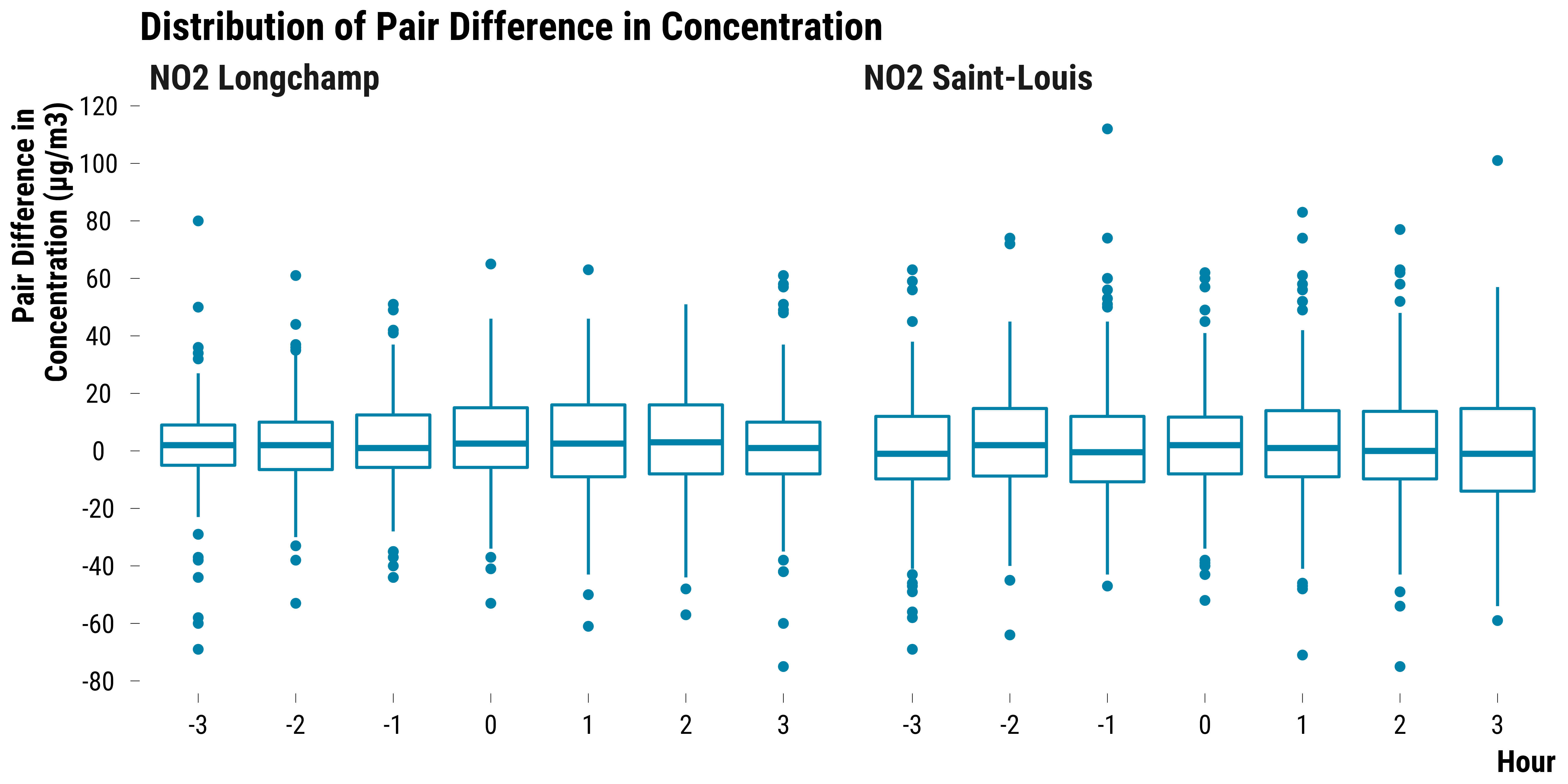
Pairs Differences in NO2 Concentrations

Boxplots for NO2:

Please show me the code!

# create the graph for no2
graph_boxplot_difference_pollutant_no2 <-
  data_pair_difference_pollutant %>%
  filter(str_detect(pollutant, "NO2")) %>%
  ggplot(., aes(x = as.factor(time), y = difference)) +
  geom_boxplot(colour = my_blue) +
  facet_wrap( ~ pollutant) +
  scale_y_continuous(breaks = scales::pretty_breaks(n = 10)) +
  ggtitle("Distribution of Pair Difference in Concentration") +
  ylab("Pair Difference in \nConcentration (µg/m3)") + xlab("Hour") +
  theme_tufte()

# display the graph
graph_boxplot_difference_pollutant_no2

Please show me the code!

# save the graph
graph_boxplot_difference_pollutant_no2 <-
  graph_boxplot_difference_pollutant_no2 +
  theme(plot.title = element_blank())

ggsave(
  graph_boxplot_difference_pollutant_no2,
  filename = here::here(
    "inputs",
    "3.outputs",
    "1.hourly_analysis",
    "2.experiment_cruise",
    "2.matching_results",
    "graph_boxplot_difference_pollutant_no2.pdf"
  ),
  width = 40,
  height = 18,
  units = "cm",
  device = cairo_pdf
)

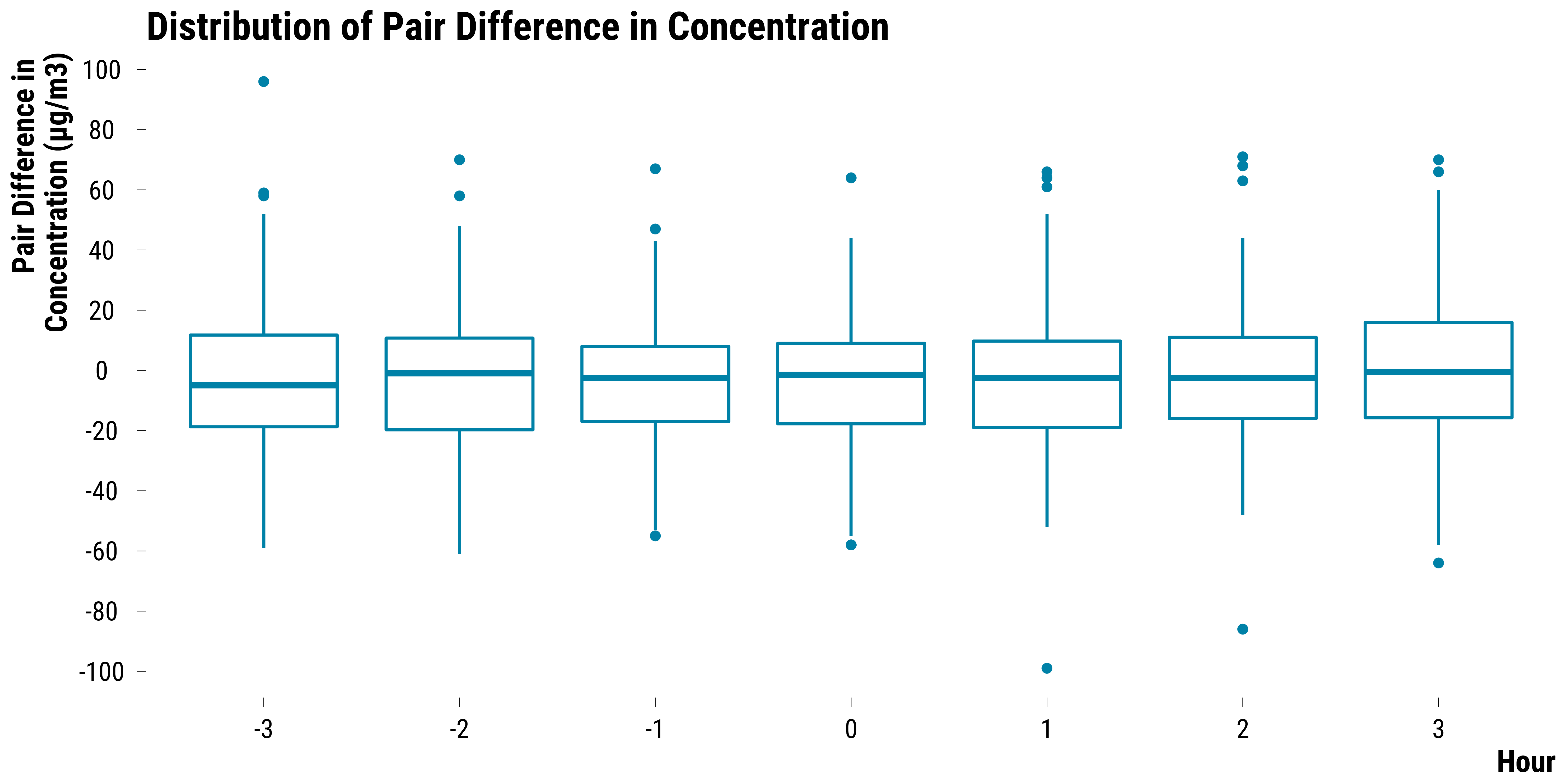
Pairs Differences in O3 Concentrations

Boxplots for O3:

Please show me the code!

# create the graph for o3
graph_boxplot_difference_pollutant_o3 <-
  data_pair_difference_pollutant %>%
  filter(str_detect(pollutant, "O3")) %>%
  ggplot(., aes(x = as.factor(time), y = difference)) +
  geom_boxplot(colour = my_blue) +
  scale_y_continuous(breaks = scales::pretty_breaks(n = 10)) +
  ggtitle("Distribution of Pair Difference in Concentration") +
  ylab("Pair Difference in \nConcentration (µg/m3)") + xlab("Hour") +
  theme_tufte()

# display the graph
graph_boxplot_difference_pollutant_o3

Please show me the code!

# save the graph
graph_boxplot_difference_pollutant_o3 <-
  graph_boxplot_difference_pollutant_o3 +
  theme(plot.title = element_blank())

ggsave(
  graph_boxplot_difference_pollutant_o3,
  filename = here::here(
    "inputs",
    "3.outputs",
    "1.hourly_analysis",
    "2.experiment_cruise",
    "2.matching_results",
    "graph_boxplot_difference_pollutant_o3.pdf"
  ),
  width = 30,
  height = 15,
  units = "cm",
  device = cairo_pdf
)

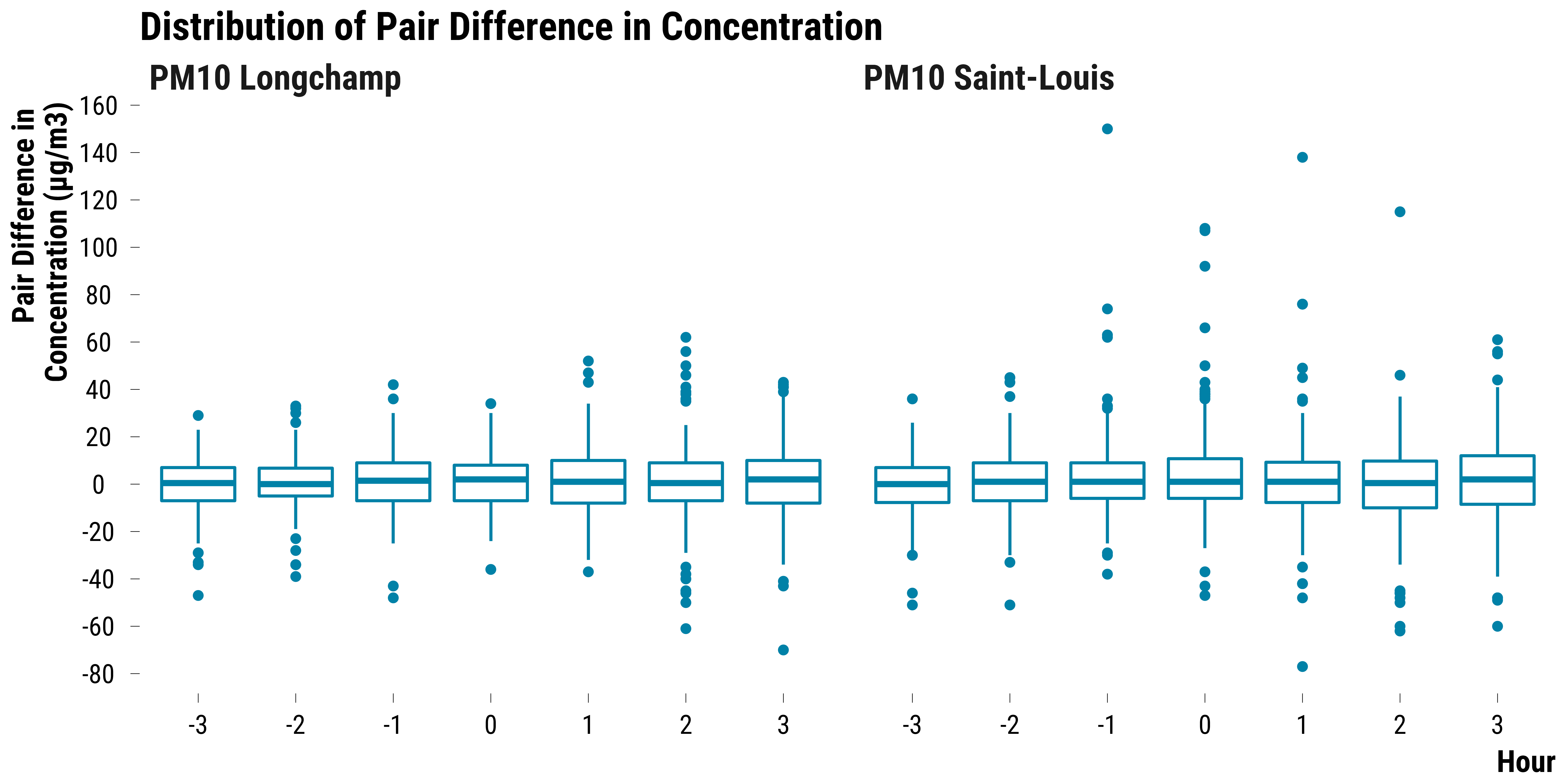
Pairs Differences in PM10 Concentrations

Boxplots for PM10:

Please show me the code!

# create the graph for pm10
graph_boxplot_difference_pollutant_pm10 <-
  data_pair_difference_pollutant %>%
  filter(str_detect(pollutant, "PM10")) %>%
  ggplot(., aes(x = as.factor(time), y = difference)) +
  geom_boxplot(colour = my_blue) +
  scale_y_continuous(breaks = scales::pretty_breaks(n = 10)) +
  facet_wrap(~ pollutant) +
  ggtitle("Distribution of Pair Difference in Concentration") +
  ylab("Pair Difference in \nConcentration (µg/m3)") + xlab("Hour") +
  theme_tufte()

# display the graph
graph_boxplot_difference_pollutant_pm10

Please show me the code!

# save the graph
graph_boxplot_difference_pollutant_pm10 <-
  graph_boxplot_difference_pollutant_pm10 +
  theme(plot.title = element_blank())

ggsave(
  graph_boxplot_difference_pollutant_pm10,
  filename = here::here(
    "inputs",
    "3.outputs",
    "1.hourly_analysis",
    "2.experiment_cruise",
    "2.matching_results",
    "graph_boxplot_difference_pollutant_pm10.pdf"
  ),
  width = 40,
  height = 18,
  units = "cm",
  device = cairo_pdf
)

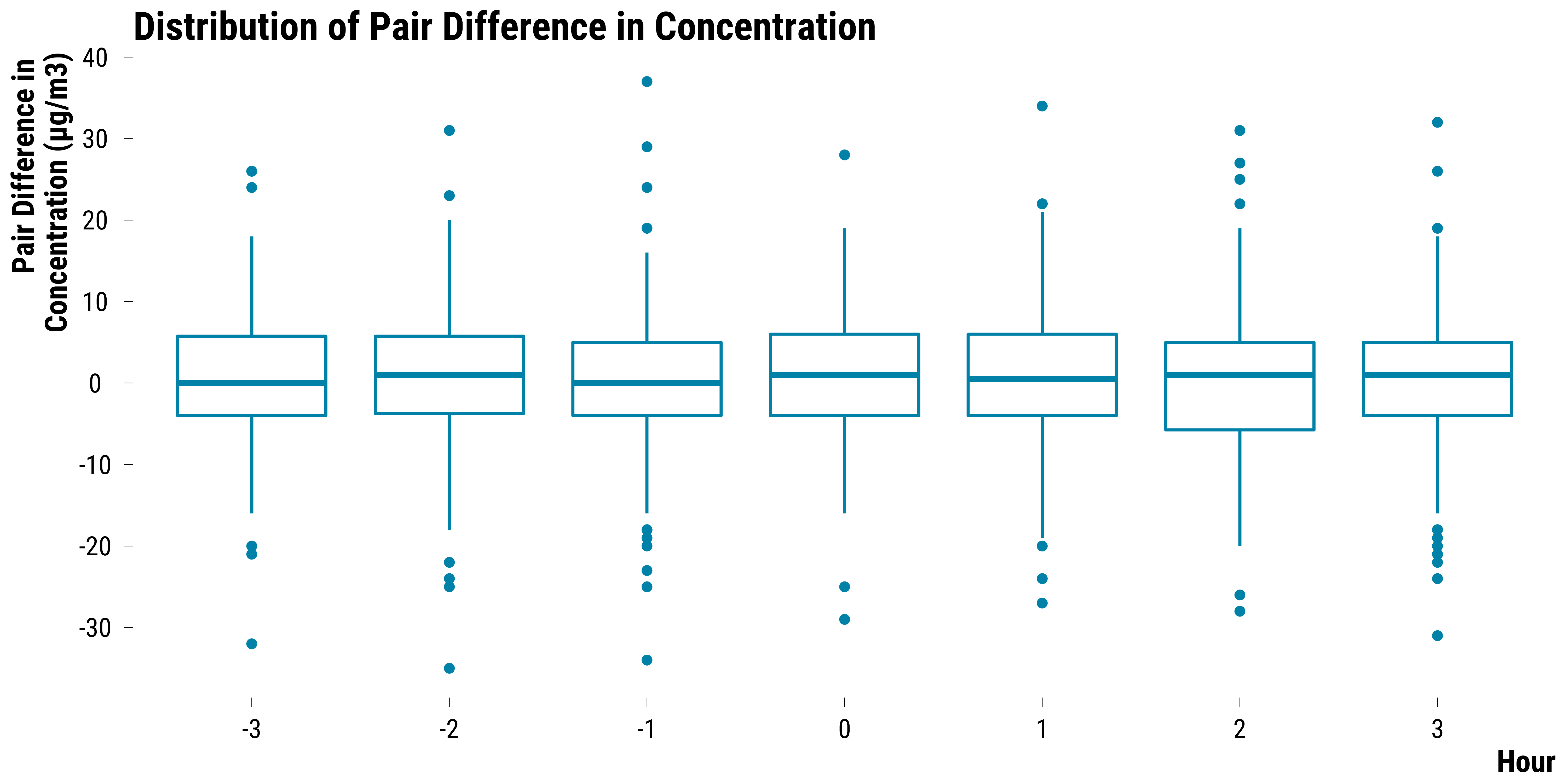
Pairs Differences in PM2.5 Concentrations

Boxplots for PM2.5:

Please show me the code!

# create the graph for pm2.5
graph_boxplot_difference_pollutant_pm25 <-
  data_pair_difference_pollutant %>%
  filter(str_detect(pollutant, "PM2.5")) %>%
  ggplot(., aes(x = as.factor(time), y = difference)) +
  geom_boxplot(colour = my_blue) +
  scale_y_continuous(breaks = scales::pretty_breaks(n = 10)) +
  ggtitle("Distribution of Pair Difference in Concentration") +
  ylab("Pair Difference in \nConcentration (µg/m3)") + xlab("Hour") +
  theme_tufte()

# display the graph
graph_boxplot_difference_pollutant_pm25

Please show me the code!

# save the graph
graph_boxplot_difference_pollutant_pm25 <-
  graph_boxplot_difference_pollutant_pm25 +
  theme(plot.title = element_blank())

ggsave(
  graph_boxplot_difference_pollutant_pm25,
  filename = here::here(
    "inputs",
    "3.outputs",
    "1.hourly_analysis",
    "2.experiment_cruise",
    "2.matching_results",
    "graph_boxplot_difference_pollutant_pm25.pdf"
  ),
  width = 30,
  height = 15,
  units = "cm",
  device = cairo_pdf
)

Pairs Differences in SO2 Concentrations

Boxplots for SO2:

Please show me the code!

# create the graph for so2
graph_boxplot_difference_pollutant_so2 <-
  data_pair_difference_pollutant %>%
  filter(str_detect(pollutant, "SO2")) %>%
  ggplot(., aes(x = as.factor(time), y = difference)) +
  geom_boxplot(colour = my_blue) +
  scale_y_continuous(breaks = scales::pretty_breaks(n = 10)) +
  ggtitle("Distribution of Pair Difference in Concentration") +
  ylab("Pair Difference in \nConcentration (µg/m3)") + xlab("Hour") +
  theme_tufte()

# display the graph
graph_boxplot_difference_pollutant_so2

Please show me the code!

# save the graph
graph_boxplot_difference_pollutant_so2 <-
  graph_boxplot_difference_pollutant_so2 +
  theme(plot.title = element_blank())

ggsave(
  graph_boxplot_difference_pollutant_so2,
  filename = here::here(
    "inputs",
    "3.outputs",
    "1.hourly_analysis",
    "2.experiment_cruise",
    "2.matching_results",
    "graph_boxplot_difference_pollutant_so2.pdf"
  ),
  width = 30,
  height = 15,
  units = "cm",
  device = cairo_pdf
)

Testing the Sharp Null Hypothesis

We test the sharp null hypothesis of no effect for any units. We first create a dataset where we nest the pair differences by pollutant and time. We also compute the observed test statistic which is the observed average of pair differences:

# nest the data by pollutant and time
ri_data_sharp_null <- data_pair_difference_pollutant   %>%
  select(pollutant, time, difference) %>%
  group_by(pollutant, time) %>%
  mutate(observed_mean_difference = mean(difference)) %>%
  group_by(pollutant, time, observed_mean_difference) %>%
  summarise(data_difference = list(difference))

We then create a function to compute the randomization distribution of the test statistic:

# randomization distribution function
# this function takes the vector of pair differences
# and then compute the average pair difference according
# to the permuted treatment assignment
function_randomization_distribution <- function(data_difference) {
  randomization_distribution = NULL
  n_columns = dim(permutations_matrix)[2]
  for (i in 1:n_columns) {
    randomization_distribution[i] =  sum(data_difference * permutations_matrix[, i]) / number_pairs
  }
  return(randomization_distribution)
}

We store the number of pairs and the number of simulations we want to run:

# define number of pairs in the experiment
number_pairs <- nrow(data_matched)/2

# define number of simulations
number_simulations <- 100000

We compute the permutations matrix:

# set the seed
set.seed(42)

# compute the permutations matrix
permutations_matrix <- matrix(rbinom(number_pairs*number_simulations, 1,.5)*2-1, nrow = number_pairs, ncol = number_simulations)

For each pollutant and time, we compute the randomization distribution of the test statistic using 100,000 iterations. It took us 46 seconds to run this code chunck on our basic local computer:

# compute the test statistic distribution
ri_data_sharp_null <- ri_data_sharp_null %>%
  mutate(randomization_distribution = map(data_difference, ~ function_randomization_distribution(.)))

Using the observed value of the test statistic and its randomization distribution, we compute the two-sided p-values:

# function to compute the upper one-sided p-value
function_fisher_upper_p_value <- function(observed_mean_difference, randomization_distribution){
  sum(randomization_distribution >= observed_mean_difference)/number_simulations
}

# function compute the lower one-sided p-value
function_fisher_lower_p_value <- function(observed_mean_difference, randomization_distribution){
  sum(randomization_distribution <= observed_mean_difference)/number_simulations
}

# compute the lower and upper one-sided p-values
ri_data_sharp_null <- ri_data_sharp_null %>%
  mutate(p_value_upper = map2_dbl(observed_mean_difference, randomization_distribution, ~ function_fisher_upper_p_value(.x, .y)),
         p_value_lower = map2_dbl(observed_mean_difference, randomization_distribution, ~ function_fisher_lower_p_value(.x, .y)))

# compute the two-sided p-value using rosenbaum (2010) procedure
ri_data_sharp_null <- ri_data_sharp_null %>%
  rowwise() %>%
  mutate(two_sided_p_value = min(c(p_value_upper, p_value_lower))*2) %>%
  mutate(two_sided_p_value = min(two_sided_p_value, 1)) %>%
  select(pollutant, time, observed_mean_difference, two_sided_p_value) %>%
  ungroup()

We plot below the two-sided p-values for the sharp null hypothesis for each pollutant:

Please show me the code!

# make the graph
graph_p_values <- ri_data_sharp_null %>%
  ggplot(., aes(x = as.factor(time), y = two_sided_p_value)) +
  geom_segment(aes(
    x = as.factor(time),
    xend = as.factor(time),
    y = 0,
    yend = two_sided_p_value
  )) +
  geom_point(
    shape = 21,
    size = 4,
    colour = "black",
    fill = my_blue
  ) +
  facet_wrap( ~ pollutant, ncol = 4) +
  xlab("Hour") + ylab("Two-Sided P-Value") +
  theme_tufte()

# display the graph
graph_p_values

Please show me the code!

# save the graph
ggsave(
  graph_p_values,
  filename = here::here(
    "inputs",
    "3.outputs",
    "1.hourly_analysis",
    "2.experiment_cruise",
    
    "2.matching_results",
    "graph_p_values.pdf"
  ),
  width = 60,
  height = 25,
  units = "cm",
  device = cairo_pdf
)

We display below the table of Fisher p-values:

Please show me the code!

ri_data_sharp_null %>%
  select(pollutant, time, observed_mean_difference, two_sided_p_value) %>%
  mutate(observed_mean_difference = round(observed_mean_difference, 1)) %>%
  rename(
    "Pollutant" = pollutant,
    "Time" = time,
    "Observed Value of the Test Statistic" = observed_mean_difference,
    "Two-Sided P-Values" = two_sided_p_value
  ) %>%
  rmarkdown::paged_table(.)

Computing Fisherian intervals

To quickly compute 95% Fisherian intervals, we run the procedure on an Amazon Web Services virtual computer (EC2 t3.2xlarge). It took about 38 minutes for the code to run. It can be found in the script_aws_fisherian_intervals.R file. We explain below how we proceed. We first create a nested dataset with the pair differences for each pollutant and hour. We also add the set of hypothetical constant effects.

# create a nested dataframe with 
# the set of constant treatment effect sizes
# and the vector of observed pair differences
ri_data_fi <- data_pair_difference_pollutant %>%
  select(pollutant, time, difference) %>%
  group_by(pollutant, time) %>%
  summarise(data_difference = list(difference)) %>%
  group_by(pollutant, time, data_difference) %>%
  expand(effect = seq(from = -10, to = 10, by = 0.1)) %>%
  ungroup()

We then substract for each pair difference the hypothetical constant effect:

# function to get the observed statistic
adjusted_pair_difference_function <- function(pair_differences, effect){
  adjusted_pair_difference <- pair_differences-effect
  return(adjusted_pair_difference)
} 

# compute the adjusted pair differences
ri_data_fi <- ri_data_fi %>%
  mutate(data_adjusted_pair_difference = map2(data_difference, effect, ~ adjusted_pair_difference_function(.x, .y)))

We compute the observed mean of adjusted pair differences:

# compute the observed mean of adjusted pair differences
ri_data_fi <- ri_data_fi %>%
  mutate(observed_mean_difference = map(data_adjusted_pair_difference, ~ mean(.))) %>%
  unnest(cols = c(observed_mean_difference)) %>%
  select(-data_difference) %>%
  ungroup()

We use the same function_randomization_distribution to compute the randomization distribution of the test statistic and run 100,000 iterations for each pollutant-hour observation:

# define number of pairs in the experiment
number_pairs <- nrow(data_matched)/2

# define number of simulations
number_simulations <- 100000

# compute the permutations matrix
permutations_matrix <- matrix(rbinom(number_pairs*number_simulations, 1,.5)*2-1, nrow = number_pairs, ncol = number_simulations)

# randomization distribution function
# this function takes the vector of pair differences
# and then compute the average pair difference according 
# to the permuted treatment assignment
function_randomization_distribution <- function(data_difference) {
  randomization_distribution = NULL
  n_columns = dim(permutations_matrix)[2]
  for (i in 1:n_columns) {
    randomization_distribution[i] =  sum(data_difference * permutations_matrix[, i]) / number_pairs
  }
  return(randomization_distribution)
}

We run the function:

# compute the test statistic distribution
ri_data_fi <- ri_data_fi %>%
  mutate(randomization_distribution = map(data_adjusted_pair_difference, ~ function_randomization_distribution(.)))

We compute the lower and upper p-values functions. From these functions, we retrieve the lower and upper bound of the 95% Fisherian intervals:

# define the p-values functions
function_fisher_upper_p_value <- function(observed_mean_difference, randomization_distribution){
  sum(randomization_distribution >= observed_mean_difference)/number_simulations
}

function_fisher_lower_p_value <- function(observed_mean_difference, randomization_distribution){
  sum(randomization_distribution <= observed_mean_difference)/number_simulations
}

# compute the lower and upper one-sided p-values
ri_data_fi <- ri_data_fi %>%
  mutate(p_value_upper = map2_dbl(observed_mean_difference, randomization_distribution, ~ function_fisher_upper_p_value(.x, .y)),
         p_value_lower = map2_dbl(observed_mean_difference, randomization_distribution, ~ function_fisher_lower_p_value(.x, .y)))

# retrieve the constant effects with the p-values equal or the closest to 0.025
ri_data_fi <- ri_data_fi %>%
  mutate(p_value_upper = abs(p_value_upper - 0.025),
         p_value_lower = abs(p_value_lower - 0.025)) %>%
  group_by(pollutant, time) %>%
  filter(p_value_upper == min(p_value_upper) | p_value_lower == min(p_value_lower)) %>%
# in case two effect sizes have a p-value equal to 0.025, we take the effect size
# that make the Fisherian interval wider to be conservative
  summarise(lower_fi = min(effect),
            upper_fi = max(effect))

We finally compute the point estimates of the Fisherian intervals which we define as the observed average of pair differences:

# compute observed average of pair differences
ri_data_fi_point_estimate <- data_pair_difference_pollutant   %>%
  select(pollutant, time, difference) %>%
  group_by(pollutant, time) %>%
  mutate(observed_mean_difference = mean(difference)) %>%
  ungroup()

We merge the point estimates data with the Fisherian intervals data:

# merge ri_data_fi_point_estimate with ri_data_fi
ri_data_fi_final <- left_join(ri_data_fi, ri_data_fi_point_estimate, by = c("pollutant", "time"))

We plot below the 95% Fisherian intervals:

Please show me the code!

# open the data on fisherian intervals
ri_data_fi_final <-
  readRDS(
    here::here(
     "inputs",
      "1.data",
      "1.hourly_data",
      "2.data_for_analysis",
      "1.matched_data",
      "ri_data_fisherian_intervals.rds"
    )
  )

# create an indicator to alternate shading of confidence intervals
ri_data_fi_final <- ri_data_fi_final %>%
  arrange(pollutant, time) %>%
  mutate(stripe = ifelse((time %% 2) == 0, "Grey", "White")) %>%
  ungroup()

# make the graph
graph_fisherian_intervals <-
  ggplot(ri_data_fi_final,
         aes(x = as.factor(time), y = observed_mean_difference)) +
  geom_rect(
    aes(fill = stripe),
    xmin = as.numeric(as.factor(ri_data_fi_final$time)) - 0.42,
    xmax = as.numeric(as.factor(ri_data_fi_final$time)) + 0.42,
    ymin = -Inf,
    ymax = Inf,
    color = NA,
    alpha = 0.4
  ) +
  geom_hline(yintercept = 0, color = "black") +
  geom_vline(xintercept = c(3.6), color = "black") +
  geom_pointrange(
    aes(
      x = as.factor(time),
      y = observed_mean_difference,
      ymin = lower_fi ,
      ymax = upper_fi
    ),
    colour = my_blue,
    lwd = 0.8
  ) +
  facet_wrap( ~ pollutant, ncol = 4) +
  scale_y_continuous(breaks = scales::pretty_breaks(n = 10)) +
  scale_fill_manual(values = c('gray80', "NA")) +
  guides(fill = FALSE) +
  ylab("Constant-Additive Increase \nin Concentrations (µg/m³)") + xlab("Hour") +
  theme_tufte()

# print the graph
graph_fisherian_intervals

Please show me the code!

# save the graph
ggsave(
  graph_fisherian_intervals,
  filename = here::here(
    "inputs",
    "3.outputs",
    "1.hourly_analysis",
    "2.experiment_cruise",
    
    "2.matching_results",
    "graph_fisherian_intervals.pdf"
  ),
  width = 35,
  height = 15,
  units = "cm",
  device = cairo_pdf
)

We display below the table with the 95% Fisherian intervals and the point estimates:

Please show me the code!

ri_data_fi_final %>%
  select(pollutant, time, observed_mean_difference, lower_fi, upper_fi) %>%
  mutate(observed_mean_difference = round(observed_mean_difference, 1)) %>%
  rename(
    "Pollutant" = pollutant,
    "Time" = time,
    "Point Estimate" = observed_mean_difference,
    "Lower Bound of the 95% Fisherian Interval" = lower_fi,
    "Upper Bound of the 95% Fisherian Interval" = upper_fi
  ) %>%
  rmarkdown::paged_table(.)

Checking the Robustness of Results

In this section, we carry out several robustness checks:

We evaluate to which extent our results could suffer from hidden bias. We first implement a sensitivity analysis for hidden bias à la Rosenbaum.
We check how our results are sensitive to outliers by computing 95% Fisherian intervals based on the Wilcoxon’s signed rank test statistic.
As we imputed the missing pollutant concentrations, we also want to see how our results might differ for the non-missing outcomes.
We compute confidence intervals for the average treatment effect using Neyman’s approach.
We finally explore how our study could suffer from type S and M errors due to low statistical power.

Sensitivity to Hidden Bias

We implement the studentized sensitivity analysis for the ATE developed by Colin B. Fogarty (2019). We first load the relevant functions:

# load fogarty's studentized Sensitivity Analysis functions
# retrieved from http://www.mit.edu/~cfogarty/StudentizedSensitivity.R

#' StudentizedSensitivity
#'Function to perform a Studentized Sensitivity analysis on the sample average treatment
#'effect in a paired observational study
#'
#' @param PairedDiff: Vector of treated-minus-control paired differences.
#' @param null: Value of the sample average treatment effect under the null.
#' @param alpha: Desired Type I error rate.
#' @param alternative: Can be "less", "greater", or "two.sided".
#' @param Gamma: Vector of values for Gamma at which to perform the sensitivity
#'  analysis.
#' @param nperm: Number of permutations to perform permutation test.
#' @param Changepoint: If true, function returns the maximal Gamma for which the
#' test rejects at level alpha.
#' @param SensitivityInterval: If true, function returns (100-alpha) sensitivity
#' intervals. They will be one-sided if the alternative is less than or greater than,
#' and two-sided if the alternative is two-sided.
#'
#' @return Gamma: Vector of Gammas for which the sensitivity analysis was performed.
#' @return pval: P-values for each value of Gamma.
#' @return GammaPval: Matrix combining Gamma and pval.
#' @return Changepoint: Maximal Gamma for which the test rejected at level alpha.
#' @return SensitivityInterval: Upper and lower bounds for 100(1-alpha) sensitivity
#' intervals for each value of Gamma.
#' @export


StudentizedSensitivity = function(PairedDiff, null = 0, alpha = 0.05, alternative = "greater", Gamma = 1, nperm = 50000, Changepoint = T, SensitivityInterval = T)
{
   if(any(Gamma < 1))
   {
     stop("Values for Gamma must be >= 1")
   }
   if(alternative!="less" & alternative!= "greater" & alternative != "two.sided")
   {
     stop("Values for alternative are `less', `greater', or `two.sided'")
   }
   if(length(null) > 1)
   {
     stop("Value under the null must be a scalar")
   }
      if(alpha < 0 | alpha > 0.5)
   {
     stop("alpha must be between 0 and 0.5")
      }

  PairedDifftrue <- PairedDiff
  alphatrue <- alpha
  I <- length(PairedDiff)
  Adjust <- PairedDiff - null

  if(alternative == "less")
  {
    Adjust <- -Adjust
  }
  if(alternative == "two.sided")
  {
    alpha <- alphatrue/2

    if(mean(Adjust) < 0)
    {
      Adjust <- -Adjust
    }
  }

  pval <- rep(0, length(Gamma))

  for(i in 1:length(Gamma))

  {
  D <- (Adjust) - (Gamma[i]-1)/(1+Gamma[i])*abs(Adjust)
  obs <- mean(D)/(sd(D)/sqrt(I))
  Adjmat <- matrix(abs(Adjust), I, nperm)
  Zmat <- matrix(runif(I*nperm) < Gamma[i]/(1+Gamma[i]), I, nperm)
  Dmat <- (2*Zmat-1)*(Adjmat) - (Gamma[i]-1)/(1+Gamma[i])*Adjmat
  perm <- colMeans(Dmat)/(sqrt(colVars(Dmat)/I))
  pval[i] <- (1+sum(perm>=obs))/(nperm + 1)
  }
  pvalret = pval
  if(alternative == "two.sided")
  {
    pvalret = 2*pval
  }
  Pmatrix <- cbind(Gamma, pvalret)
  colnames(Pmatrix) <- c("Gamma", "P-value")

  if(Changepoint == T)
  {
    proceed <- StudentizedSensitivity(PairedDifftrue, null, alphatrue, alternative, Gamma=1, nperm,
                                      Changepoint = F, SensitivityInterval = F)$pval <= alphatrue

    change <- 1

    if(proceed)
    {
      change <- uniroot(StudentizedChangepoint, interval = c(1, 30), PairedDiff = PairedDifftrue, null = null,
                        alpha = alphatrue, alternative = alternative, nperm = nperm,
                        extendInt = "upX")$root
    }
  }

  if(SensitivityInterval == T)
    {
      lb = rep(-Inf, length(Gamma))
      ub = rep(Inf, length(Gamma))
      for(i in 1:length(Gamma))
      {
        # Warm Starts
      UB = uniroot(BoundFinder, PairedDifftrue, Gamma[i],
                   interval = c(mean(PairedDifftrue), mean(PairedDifftrue)+4*sd(PairedDifftrue)/sqrt(I)), extendInt = "yes")$root
      LB = -uniroot(BoundFinder, -PairedDifftrue, Gamma[i],
                    interval = c(-mean(PairedDifftrue)-4*sd(PairedDifftrue)/sqrt(I), -mean(PairedDifftrue)), extendInt = "yes")$root

      SUB = Inf
      SLB = -Inf

      if(alternative == "greater")
      {
        SLB = uniroot(StudentizedSI, interval = c(UB-4*sd(PairedDifftrue)/sqrt(I), UB), extendInt = "yes",
                      Gamma = Gamma[i], PairedDiff=PairedDifftrue, alternative = "greater", alpha = alpha, nperm = nperm)$root
      }

      if(alternative == "less")
      {
        SUB = uniroot(StudentizedSI, interval = c(LB, LB + 4*sd(PairedDifftrue)/sqrt(I)), extendInt = "yes",
                      Gamma = Gamma[i], PairedDiff=PairedDifftrue, alternative = "less", alpha = alpha, nperm = nperm)$root
      }

      if(alternative == "two.sided")
      {
       SLB = uniroot(StudentizedSI, interval = c(UB-4*sd(PairedDifftrue)/sqrt(I), UB), extendInt = "yes",
                     Gamma = Gamma[i], PairedDiff=PairedDifftrue, alternative = "greater", alpha = alpha, nperm = nperm)$root
       SUB = uniroot(StudentizedSI, interval = c(LB, LB+4*sd(PairedDifftrue)/sqrt(I)), extendInt = "yes",
                     Gamma = Gamma[i], PairedDiff=PairedDifftrue, alternative = "less", alpha = alpha, nperm = nperm)$root
      }

      lb[i] = SLB
      ub[i] = SUB
      }

    SImat = cbind(Gamma, lb, ub)
    colnames(SImat) = c("Gamma", "Lower Bound", "Upper Bound")
    }
    if(Changepoint == F & SensitivityInterval == F)
    {
      return(list(Gamma=Gamma, pval = pvalret, GammaPval = Pmatrix))
    }
    if(Changepoint == F & SensitivityInterval == T)
    {
      return(list(Gamma = Gamma, pval = pvalret, GammaPval = Pmatrix, SensitivityInterval = SImat))
    }
    if(Changepoint == T & SensitivityInterval == F)
    {
      return(list(Gamma = Gamma, pval = pvalret, GammaPval = Pmatrix, Changepoint = change))
    }
    if(Changepoint == T & SensitivityInterval == T)
    {
      return(list(Gamma = Gamma, pval = pvalret, GammaPval = Pmatrix, Changepoint = change,
                  SensitivityInterval = SImat))
    }

}

####These are auxiliary functions used for root finding and for calculating columnwise variances in StudentizedSensitivity
StudentizedChangepoint = function(Gamma, PairedDiff, null, alternative, alpha, nperm)
{
  alphachange = alpha
  StudentizedSensitivity(PairedDiff, null, alpha, alternative, Gamma, nperm, Changepoint = F, SensitivityInterval = F)$pval - alphachange
}

StudentizedSI = function(null,  Gamma, PairedDiff,  alternative, alpha, nperm)
{
  StudentizedSensitivity(PairedDiff, null, alpha, alternative, Gamma, nperm, Changepoint = F, SensitivityInterval = F)$pval - alpha
}

BoundFinder = function(null,  PairedDiff, Gamma)
{
  mean(PairedDiff - null - (Gamma-1)/(1+Gamma)*abs(PairedDiff-null))
}

colVars <- function(x) {
  N = nrow(x)
  (colSums(x^2) - colSums(x)^2/N) / (N-1)
}

We select the pair differences for NO\(_{2}\) in Longchamp and PM\(_{10}\) in Saint-Louis concentrations in t and run the function for \(\Gamma=2\):

# we select the relevant pair differences
data_hidden_bias <- data_pair_difference_pollutant %>%
  filter(pollutant %in% c("NO2 Longchamp", "PM10 Saint-Louis") &
           time == 0) %>%
  select(pollutant, difference) %>%
  group_by(pollutant) %>%
  nest() %>%
  mutate(data = map(data, ~ unlist(.)))

data_hidden_bias %>%
  mutate(
    sensitivity_interval = map(
      data,
      ~ StudentizedSensitivity(
        .,
        null = 0,
        alpha = 0.05,
        alternative = "two.sided",
        Gamma = 1.5,
        nperm = 10000,
        Changepoint = T,
        SensitivityInterval = T
      )$SensitivityInterval %>% as_tibble(.)
    )
  ) %>%
  select(-data) %>%
  unnest(cols = c(sensitivity_interval)) %>%
  mutate_at(vars(-pollutant), ~ round(., 2)) %>%
  kable(., align = c("l", rep("c", 3))) %>%
  kableExtra::kable_styling(position = "center")

pollutant	Gamma	Lower Bound	Upper Bound
NO2 Longchamp	1.5	-1.48	11.37
PM10 Saint-Louis	1.5	-1.87	12.17

Outliers

To gauge how sensitive our results are to outliers, we use a Wilcoxon signed rank test statistic and compute 95% Fisherian intervals using the wilcox.test() function.

Please show me the code!

# carry out the wilcox.test
data_rank_ci <- data_pair_difference_pollutant %>%
  select(-pair_number) %>%
  group_by(pollutant, time) %>%
  nest() %>%
  mutate(
    effect = map(data, ~ wilcox.test(.$difference, conf.int = TRUE)$estimate),
    lower_ci = map(data, ~ wilcox.test(.$difference, conf.int = TRUE)$conf.int[1]),
    upper_ci = map(data, ~ wilcox.test(.$difference, conf.int = TRUE)$conf.int[2])
  ) %>%
  unnest(cols = c(effect, lower_ci, upper_ci)) %>%
  mutate(data = "Wilcoxon Rank Test Statistic")

# bind ri_data_fi_final with data_rank_ci
data_ci <- ri_data_fi_final %>%
  rename(effect = observed_mean_difference,
         lower_ci = lower_fi,
         upper_ci = upper_fi) %>%
  mutate(data = "Average Pair Difference Test Statistic") %>%
  bind_rows(., data_rank_ci)

# create an indicator to alternate shading of confidence intervals
data_ci <- data_ci %>%
  arrange(pollutant, time) %>%
  mutate(stripe = ifelse((time %% 2) == 0, "Grey", "White")) %>%
  ungroup()

# make the graph
graph_ri_ci_wilcoxon <-
  ggplot(
    data_ci,
    aes(
      x = as.factor(time),
      y = effect,
      ymin = lower_ci,
      ymax = upper_ci,
      colour = data,
      shape = data
    )
  ) +
  geom_rect(
    aes(fill = stripe),
    xmin = as.numeric(as.factor(data_ci$time)) - 0.42,
    xmax = as.numeric(as.factor(data_ci$time)) + 0.42,
    ymin = -Inf,
    ymax = Inf,
    color = NA,
    alpha = 0.1
  ) +
  geom_hline(yintercept = 0, color = "black") +
  geom_vline(xintercept = c(3.6), color = "black") +
  geom_pointrange(position = position_dodge(width = 1),
                  size = 0.8,
                  fatten = 2) +
  scale_shape_manual(name = "Test Statistic:", values = c(16, 17)) +
  scale_color_manual(name = "Test Statistic:", values = c(my_orange, my_blue)) +
  facet_wrap( ~ pollutant, scales = "free_y", ncol = 4) +
  scale_fill_manual(values = c('gray80', "NA")) +
  guides(fill = FALSE) +
  ylab("Constant-Additive Increase \nin Concentrations (µg/m³)") + xlab("Hour") +
  theme_tufte()

# print the graph
graph_ri_ci_wilcoxon

Please show me the code!

# save the graph
ggsave(
  graph_ri_ci_wilcoxon,
  filename = here::here(
    "inputs",
    "3.outputs",
    "1.hourly_analysis",
    "2.experiment_cruise",
    "2.matching_results",
    "graph_ri_ci_wilcoxon.pdf"
  ),
  width = 40,
  height = 20,
  units = "cm",
  device = cairo_pdf
)

Missing Outcomes

We load non-imputed air pollution data and compute for each pollutant the 0-6 daily lags and leads:

# load marseille raw air pollution data
data_marseille_raw_pollutants <- readRDS(
  here::here(
    "inputs",
    "1.data",
    "1.hourly_data",
    "1.raw_data",
    "2.pollution_data",
    "marseille",
    "raw_marseille_hourly_pollutants_2008_2018_data.rds"
  )
) %>%
  rename_at(vars(-date), function(x)
    paste0("raw_", x)) %>%
  dplyr::as_data_frame()

# we first define data_marseille_raw_pollutants_leads and data_marseille_raw_pollutants_lags
# to store leads and lags

data_marseille_raw_pollutants_leads <- data_marseille_raw_pollutants
data_marseille_raw_pollutants_lags <- data_marseille_raw_pollutants

#
# create leads
#

# create a list to store dataframe of leads
leads_list <- vector(mode = "list", length = 3)
names(leads_list) <- c(1:3)

# create the leads
for (i in 1:3) {
  leads_list[[i]] <- data_marseille_raw_pollutants_leads %>%
    mutate_at(vars(-date), ~  lead(., n = i, order_by = date)) %>%
    rename_at(vars(-date), function(x)
      paste0(x, "_lead_", i))
}

# merge the dataframes of leads
data_leads <- leads_list %>%
  reduce(left_join, by = "date")

# merge the leads with the data_marseille_raw_pollutants_leads
data_marseille_raw_pollutants_leads <-
  left_join(data_marseille_raw_pollutants_leads, data_leads, by = "date") %>%
  select(-c(raw_mean_no2_l:raw_mean_pm10_sl))

#
# create lags
#

# create a list to store dataframe of lags
lags_list <- vector(mode = "list", length = 3)
names(lags_list) <- c(1:3)

# create the lags
for (i in 1:3) {
  lags_list[[i]] <- data_marseille_raw_pollutants_lags %>%
    mutate_at(vars(-date), ~  lag(., n = i, order_by = date)) %>%
    rename_at(vars(-date), function(x)
      paste0(x, "_lag_", i))
}

# merge the dataframes of lags
data_lags <- lags_list %>%
  reduce(left_join, by = "date")

# merge the lags with the initial data_marseille_raw_pollutants_lags
data_marseille_raw_pollutants_lags <-
  left_join(data_marseille_raw_pollutants_lags, data_lags, by = "date")

#
# merge data_marseille_raw_pollutants_leads with data_marseille_raw_pollutants_lags
#

data_marseille_raw_pollutants <-
  left_join(data_marseille_raw_pollutants_lags,
            data_marseille_raw_pollutants_leads,
            by = "date")

We merge these data with the matched data and compute pair differences:

# merge with the matched data
data_matched_with_raw_pollutants <-
  merge(data_matched, data_marseille_raw_pollutants, by = "date")

# compute pair differences
data_matched_wide_raw_pollutants <-
  data_matched_with_raw_pollutants %>%
  mutate(is_treated = ifelse(is_treated == TRUE, "treated", "control")) %>%
  select(
    is_treated,
    pair_number,
    contains("raw_mean_no2_l"),
    contains("raw_mean_no2_sl"),
    contains("raw_mean_o3"),
    contains("raw_mean_pm10_l"),
    contains("raw_mean_pm10_sl"),
    contains("raw_mean_pm25"),
    contains("raw_mean_so2")
  ) %>%
  pivot_longer(
    cols = -c(pair_number, is_treated),
    names_to = "variable",
    values_to = "concentration"
  ) %>%
  mutate(
    pollutant = NA %>%
      ifelse(str_detect(variable, "no2_l"), "NO2 Longchamp", .) %>%
      ifelse(str_detect(variable, "no2_sl"), "NO2 Saint-Louis", .) %>%
      ifelse(str_detect(variable, "o3"), "O3 Longchamp", .) %>%
      ifelse(str_detect(variable, "pm10_l"), "PM10 Longchamp", .) %>%
      ifelse(str_detect(variable, "pm10_sl"), "PM10 Saint-Louis", .) %>%
      ifelse(str_detect(variable, "pm25"), "PM2.5 Longchamp", .) %>%
      ifelse(str_detect(variable, "so2"), "SO2 Lonchamp", .)
  ) %>%
  mutate(
    time = 0 %>%
      ifelse(str_detect(variable, "lag_1"),-1, .) %>%
      ifelse(str_detect(variable, "lag_2"),-2, .) %>%
      ifelse(str_detect(variable, "lag_3"),-3, .) %>%
      ifelse(str_detect(variable, "lead_1"), 1, .) %>%
      ifelse(str_detect(variable, "lead_2"), 2, .) %>%
      ifelse(str_detect(variable, "lead_3"), 3, .)
  ) %>%
  select(-variable) %>%
  select(pair_number, is_treated, pollutant, time, concentration) %>%
  pivot_wider(names_from = is_treated, values_from = concentration)

data_raw_pair_difference_pollutant <-
  data_matched_wide_raw_pollutants %>%
  mutate(difference = treated - control) %>%
  select(-c(treated, control))

We display below the number of missing differences by pollutant and day:

Please show me the code!

# make the graph
graph_missing_pollutants <- data_raw_pair_difference_pollutant %>%
  group_by(pollutant, time) %>%
  summarise(n_missing = sum(is.na(difference))) %>%
  ggplot(., aes(x = as.factor(time), y = n_missing)) +
  geom_segment(aes(
    x = as.factor(time),
    xend = as.factor(time),
    y = 0,
    yend = n_missing
  )) +
  geom_point(
    shape = 21,
    size = 4,
    colour = "black",
    fill = my_blue
  ) +
  facet_wrap( ~ pollutant) +
  xlab("Day") + ylab("Number of Pairs with Missing Concentrations") +
  theme_tufte()

# display the graph
graph_missing_pollutants

Please show me the code!

# save the graph
ggsave(
  graph_missing_pollutants,
  filename = here::here(
    "inputs",
    "3.outputs",
    "1.hourly_analysis",
    "2.experiment_cruise",
    "2.matching_results",
    "graph_missing_pollutants.pdf"
  ),
  width = 40,
  height = 20,
  units = "cm",
  device = cairo_pdf
)

As we have 138 pairs, up to 25% of the pairs can have missing pollutant concentrations. We compute below the 95% Fisherian intervals for pairs without missing concentrations and compare the results to those found with the imputed dataset:

Please show me the code!

# carry out the wilcox.test
data_raw_rank_ci <- data_raw_pair_difference_pollutant %>%
  drop_na() %>%
  select(-pair_number) %>%
  group_by(pollutant, time) %>%
  nest() %>%
  mutate(
    effect = map(data, ~ wilcox.test(.$difference, conf.int = TRUE)$estimate),
    lower_ci = map(data, ~ wilcox.test(.$difference, conf.int = TRUE)$conf.int[1]),
    upper_ci = map(data, ~ wilcox.test(.$difference, conf.int = TRUE)$conf.int[2])
  ) %>%
  unnest(cols = c(effect, lower_ci, upper_ci)) %>%
  mutate(data = "Pairs without Missing Concentrations")

# bind data_rank_ci with data_raw_rank_ci
data_ci <- data_rank_ci %>%
  mutate(data = "Pairs with Imputed Pollutant Concentrations") %>%
  bind_rows(., data_raw_rank_ci)

# create an indicator to alternate shading of confidence intervals
data_ci <- data_ci %>%
  arrange(pollutant, time) %>%
  mutate(stripe = ifelse((time %% 2) == 0, "Grey", "White")) %>%
  ungroup()

# make the graph
graph_ri_ci_missing_concentration <-
  ggplot(
    data_ci,
    aes(
      x = as.factor(time),
      y = effect,
      ymin = lower_ci,
      ymax = upper_ci,
      colour = data,
      shape = data
    )
  ) +
  geom_rect(
    aes(fill = stripe),
    xmin = as.numeric(as.factor(data_ci$time)) - 0.42,
    xmax = as.numeric(as.factor(data_ci$time)) + 0.42,
    ymin = -Inf,
    ymax = Inf,
    color = NA,
    alpha = 0.1
  ) +
  geom_hline(yintercept = 0, color = "black") +
  geom_vline(xintercept = c(3.6), color = "black") +
  geom_pointrange(position = position_dodge(width = 1),
                  size = 0.8,
                  fatten = 2) +
  scale_shape_manual(name = "Dataset:", values = c(16, 17)) +
  scale_color_manual(name = "Dataset:", values = c(my_orange, my_blue)) +
  facet_wrap( ~ pollutant, scales = "free_y", ncol = 4) +
scale_fill_manual(values = c('gray80', "NA")) +
  guides(fill = FALSE) +
  ylab("Constant-Additive Increase \nin Concentrations (µg/m³)") + xlab("Hour") +
  theme_tufte()

# print the graph
graph_ri_ci_missing_concentration

Please show me the code!

# save the graph
ggsave(
  graph_ri_ci_missing_concentration,
  filename = here::here(
    "inputs",
    "3.outputs",
    "1.hourly_analysis",
    "2.experiment_cruise",
    "2.matching_results",
    "graph_ri_ci_missing_concentration.pdf"
  ),
  width = 40,
  height = 20,
  units = "cm",
  device = cairo_pdf
)

Neyman’s Approach: Computing Confidence Intervals for the Average Treatment Effects

We compute confidence intervals for the average treatement using Neyman’s approach. We use the formula for the standard error of pair randomized experiment found in Imbens and Rubin (2015).

# we first compute the average treatment effects for each pollutant and hour
data_pair_mean_difference <- data_pair_difference_pollutant %>%
  group_by(pollutant, time) %>%
  summarise(mean_difference = mean(difference)) %>%
  ungroup()

# we store the number of pairs
n_pair <- nrow(data_matched) / 2

# compute the standard error
data_se_neyman_pair <-
  left_join(
    data_pair_difference_pollutant,
    data_pair_mean_difference,
    by = c("pollutant", "time")
  ) %>%
  mutate(squared_difference = (difference - mean_difference) ^ 2) %>%
  group_by(pollutant, time) %>%
  summarise(standard_error = sqrt(1 / (n_pair * (n_pair - 1)) * sum(squared_difference))) %>%
  select(pollutant, time, standard_error) %>%
  ungroup()

# merge the average treatment effect data witht the standard error data
data_neyman <-
  left_join(data_pair_mean_difference,
            data_se_neyman_pair,
            by = c("pollutant", "time")) %>%
  # compute the 95% confidence intervals
  mutate(
    ci_lower_95 = mean_difference - 1.96 * standard_error,
    ci_upper_95 = mean_difference + 1.96 * standard_error
  ) %>%
  mutate(data = "Neyman")

# save the data
saveRDS(
  data_neyman,
  here::here(
    "inputs",
    "1.data",
    "1.hourly_data",
    "2.data_for_analysis",
    "1.matched_data",
    "data_neyman.rds"
  )
)

We plot the the point estimates for the average treatment effects and their associated 95% confidence intervals:

Please show me the code!

# bind ri_data_fi_final with data_neyman
data_ci <- ri_data_fi_final %>%
  rename(mean_difference = observed_mean_difference,
         ci_lower_95 = lower_fi,
         ci_upper_95 = upper_fi) %>%
  mutate(data = "Fisher") %>%
  bind_rows(., data_neyman)

# create an indicator to alternate shading of confidence intervals
data_ci <- data_ci %>%
  arrange(pollutant, time) %>%
  mutate(stripe = ifelse((time %% 2) == 0, "Grey", "White")) %>%
  ungroup()

# make the graph
graph_neyman_ci <-
  ggplot(
    data_ci,
    aes(
      x = as.factor(time),
      y = mean_difference,
      ymin = ci_lower_95,
      ymax = ci_upper_95,
      colour = data,
      shape = data
    )
  ) +
  geom_rect(
    aes(fill = stripe),
    xmin = as.numeric(as.factor(data_ci$time)) - 0.42,
    xmax = as.numeric(as.factor(data_ci$time)) + 0.42,
    ymin = -Inf,
    ymax = Inf,
    color = NA,
    alpha = 0.1
  ) +
  geom_hline(yintercept = 0, color = "black") +
  geom_vline(xintercept = c(3.6), color = "black") +
  geom_pointrange(position = position_dodge(width = 1),
                  size = 0.8,
                  fatten = 2) +
  scale_shape_manual(name = "Mode of Inference:", values = c(16, 17)) +
  scale_color_manual(name = "Mode of Inference:", values = c(my_orange, my_blue)) +
  facet_wrap( ~ pollutant, scales = "free_y", ncol = 4) +
  scale_fill_manual(values = c('gray80', "NA")) +
  guides(fill = FALSE) +
  ylab("Increase \nin Concentrations (µg/m³)") + xlab("Hour") +
  theme_tufte()

# print the graph
graph_neyman_ci

Please show me the code!

# save the graph
ggsave(
  graph_neyman_ci,
  filename = here::here(
    "inputs",
    "3.outputs",
    "1.hourly_analysis",
    "2.experiment_cruise",
    "2.matching_results",
    "graph_ci_neyman.pdf"
  ),
  width = 40,
  height = 20,
  units = "cm",
  device = cairo_pdf
)

Statistical Power Issues

Our matching procedure resulted in few matched treated units: we might therefore have a low statistical power to detect the effect of cruise vessels on air pollutant concentrations. Even more worrying is our higher chance to suffer from type-S an type-M errors. While we do not know what the true effect of cruise on air pollutants is, we can explore our statistical power and our probability to make types S and M errors using a grid of plausible effect sizes. We proceed as follows:

We take the standard error computed for the average treatment effect of cruise on NO2 concentration in t at Longchamp.
We set create a grid of plausible effect sizes.
The retrodesign package allows us to compute the statistical power, the type-M and type-S errors associated with each effect size.

# retrieve the standard error
standard_error <- data_neyman %>%
  filter(pollutant == "NO2 Longchamp" & time == 0) %>%
  pull(standard_error)

# create data on plausible effect sizes
data_type_m_s_errors <-
  tibble(plausible_effect = seq(from = 0.25, to = 5, by = 0.1))

# add the standard error to data_type_m_s_errors
data_type_m_s_errors <- data_type_m_s_errors %>%
  mutate(standard_error = standard_error)

# we compute power, type s and m errors
data_type_m_s_errors <- data_type_m_s_errors %>%
  mutate(
    power = map2(
      plausible_effect,
      standard_error,
      ~ retro_design(.x, .y)$power * 100
    ),
    type_m_error = map2(plausible_effect, standard_error, ~ retro_design(.x, .y)$typeM),
    type_s_error = map2(
      plausible_effect,
      standard_error,
      ~ retro_design(.x, .y)$typeS * 100
    )
  ) %>%
  unnest(c(power, type_m_error, type_s_error))

We plot and save the results:

Please show me the code!

# make the graph
graph_type_m_s_errors <- data_type_m_s_errors %>%
  rename(
    "Power (%)" = power,
    "Type M Error (Bias)" = type_m_error,
    "Type S Error (%)" = type_s_error
  ) %>%
  pivot_longer(
    cols = -c(plausible_effect, standard_error),
    names_to = "variable",
    values_to = "value"
  ) %>%
  ggplot(., aes(x = plausible_effect, y = value)) +
  geom_line(colour = my_blue) +
  geom_vline(xintercept = 4.7, colour = my_orange) +
  geom_vline(xintercept = 2.35, colour = my_orange, linetype = "dashed") +
  scale_y_continuous(breaks = scales::pretty_breaks(n = 10),limits = c(0, NA)) +
  facet_wrap(~ variable, scales = "free") +
  xlab("Plausible Effect Sizes for an Average Increase\n in NO2 Concentrations (µg/m³)") + ylab("") +
  theme_tufte()


# print the graph
graph_type_m_s_errors

Please show me the code!

# save the graph
ggsave(
  graph_type_m_s_errors,
  filename = here::here(
    "inputs",
    "3.outputs",
    "1.hourly_analysis",
    "2.experiment_cruise",
    "2.matching_results",
    "graph_type_m_s_errors.pdf"
  ),
  width = 25,
  height = 10,
  units = "cm",
  device = cairo_pdf
)

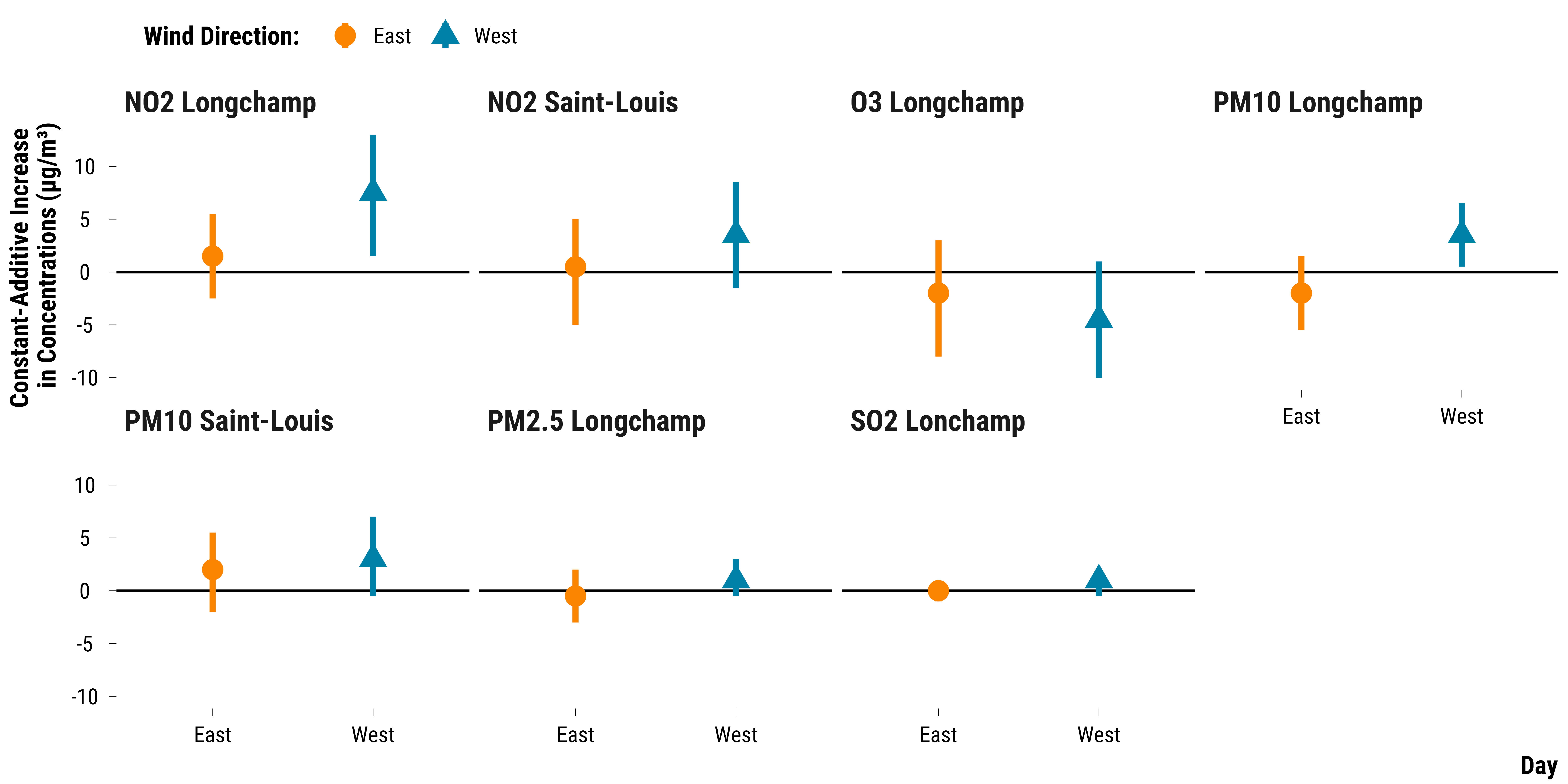
Heterogeneity Analysis

Please show me the code!

# prepare data on pair differences in concentration and wind direction
data_pair_difference_pollutant_0 <-
  data_pair_difference_pollutant %>%
  filter(time == 0)

data_pair_wd <- data_matched %>%
  select(pair_number, wind_direction_east_west) %>%
  distinct()

data_pair_difference_pollutant_0_wd <-
  left_join(data_pair_difference_pollutant_0, data_pair_wd, by = "pair_number") %>%
  select(-time, -pair_number)


# carry out the wilcox.test
data_rank_ci_wd <- data_pair_difference_pollutant_0_wd %>%
  group_by(pollutant, wind_direction_east_west) %>%
  nest() %>%
  mutate(
    effect = map(data, ~ wilcox.test(.$difference, conf.int = TRUE)$estimate),
    lower_ci = map(data, ~ wilcox.test(.$difference, conf.int = TRUE)$conf.int[1]),
    upper_ci = map(data, ~ wilcox.test(.$difference, conf.int = TRUE)$conf.int[2])
  ) %>%
  unnest(cols = c(effect, lower_ci, upper_ci)) %>%
  select(-data)


# make the graph
graph_wilcoxon_wd <-
  ggplot(
    data_rank_ci_wd,
    aes(
      x = wind_direction_east_west,
      y = effect,
      ymin = lower_ci,
      ymax = upper_ci,
      colour = wind_direction_east_west,
      shape = wind_direction_east_west
    )
  ) +
  geom_hline(yintercept = 0, color = "black") +
  geom_pointrange(position = position_dodge(width = 1), size = 1.2) +
  scale_shape_manual(name = "Wind Direction:", values = c(16, 17)) +
  scale_color_manual(name = "Wind Direction:", values = c(my_orange, my_blue)) +
  facet_wrap(~ pollutant, ncol = 4) +
  guides(fill = FALSE) +
  ylab("Constant-Additive Increase \nin Concentrations (µg/m³)") + xlab("Day") +
  theme_tufte()

# print the graph
graph_wilcoxon_wd

Please show me the code!

# save the graph
ggsave(
  graph_wilcoxon_wd,
  filename = here::here(
    "inputs",
    "3.outputs",
    "1.hourly_analysis",
    "2.experiment_cruise",
    "2.matching_results",
    "graph_wilcoxon_wd.pdf"
  ),
  width = 30,
  height = 15,
  units = "cm",
  device = cairo_pdf
)

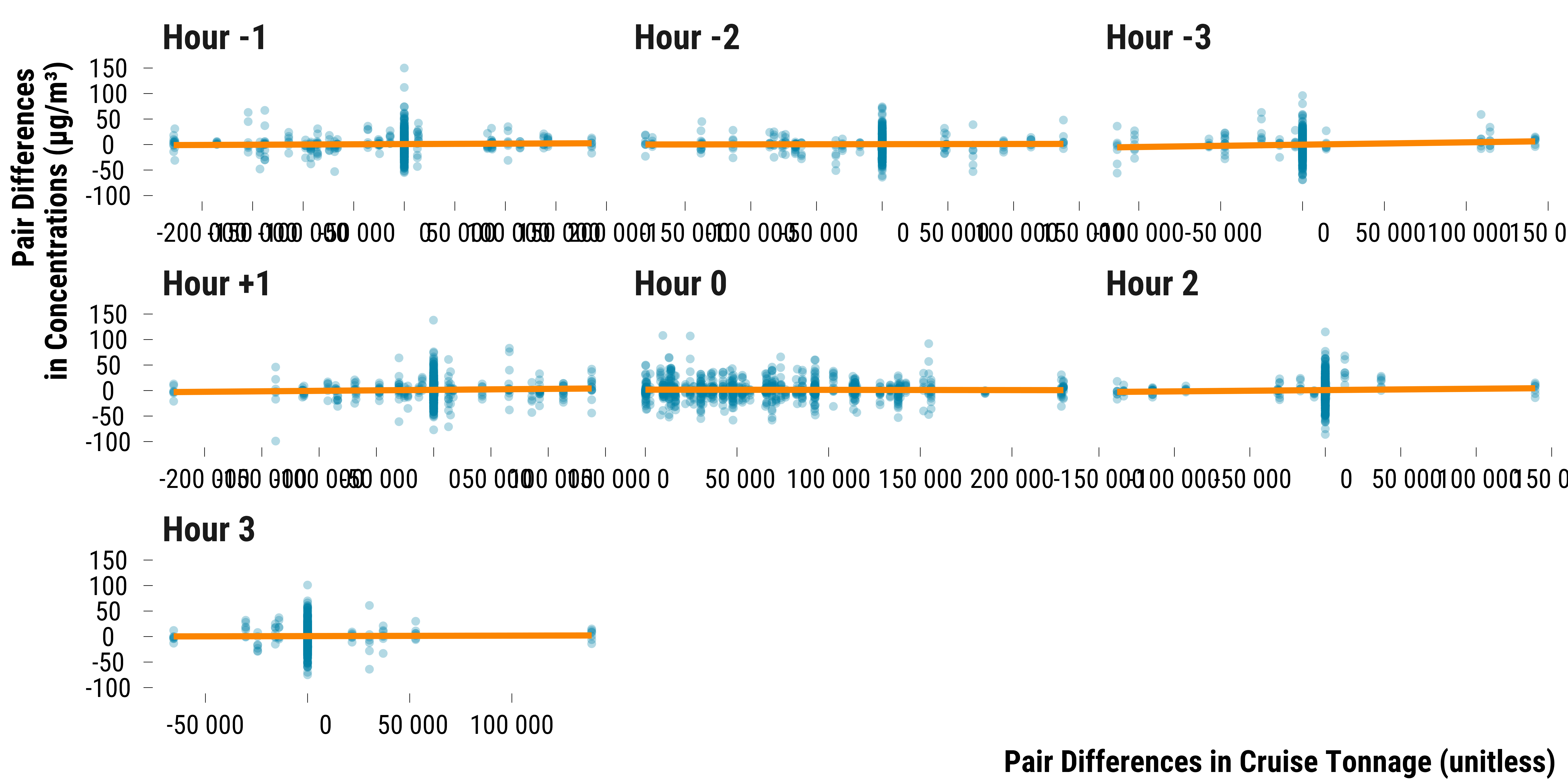
Please show me the code!

# joint concentration differences with tonnage differences
data_pair_difference_pollutant <- data_pair_difference_pollutant %>%
  rename(difference_concentration = difference)

data_matched_wide_tonnage <- data_matched %>%
  mutate(is_treated = ifelse(is_treated == TRUE, "treated", "control")) %>%
  select(is_treated,
         pair_number,
         contains("total_gross_tonnage_entry_cruise")) %>%
  pivot_longer(
    cols = -c(pair_number, is_treated),
    names_to = "variable",
    values_to = "tonnage"
  ) %>%
  mutate(
    time = 0 %>%
      ifelse(str_detect(variable, "lag_3"),-3, .) %>%
      ifelse(str_detect(variable, "lag_2"),-2, .) %>%
      ifelse(str_detect(variable, "lag_1"),-1, .) %>%
      ifelse(str_detect(variable, "lead_1"), 1, .) %>%
      ifelse(str_detect(variable, "lead_2"), 2, .) %>% 
      ifelse(str_detect(variable, "lead_3"), 3, .)
  ) %>%
  mutate(variable = "total_gross_tonnage_entry_cruise") %>%
  select(pair_number, is_treated, variable, time, tonnage) %>%
  pivot_wider(names_from = is_treated, values_from = tonnage)

data_pair_difference_tonnage <- data_matched_wide_tonnage %>%
  mutate(difference_tonnage = treated - control) %>%
  select(-c(treated, control))

data_concentration_tonnage_pair <- left_join(
  data_pair_difference_pollutant,
  data_pair_difference_tonnage,
  by = c("pair_number", "time")
) %>%
  mutate(time = ifelse(time == 1, "+1", time),
         time = paste("Hour", time, sep = " "))

# make the graph
graph_concentration_tonnage_pair <-
  data_concentration_tonnage_pair %>%
  ggplot(., aes(x =  difference_tonnage, y = difference_concentration)) +
  geom_point(shape = 16,
             colour = my_blue,
             alpha = 0.3) +
  geom_smooth(method = "lm",
              se = FALSE,
              colour = my_orange) +
  scale_x_continuous(
    breaks = scales::pretty_breaks(n = 8),
    labels = function(x)
      format(x, big.mark = " ", scientific = FALSE)
  ) +
  facet_wrap( ~ time, scales = "free_x") +
  xlab("Pair Differences in Cruise Tonnage (unitless)") + ylab("Pair Differences \nin Concentrations (µg/m³)") +
  theme_tufte()

# print the graph
graph_concentration_tonnage_pair

Please show me the code!

# save the graph
ggsave(
  graph_concentration_tonnage_pair,
  filename = here::here(
    "inputs",
    "3.outputs",
    "1.hourly_analysis",
    "2.experiment_cruise",
    "2.matching_results",
    "graph_concentration_tonnage_pair.pdf"
  ),
  width = 35,
  height = 12,
  units = "cm",
  device = cairo_pdf
)

Analyzing Results - Entering Cruise Experiment

Required Packages

Preparing the Data

Distribution of the Pair Differences in Concentration between Treated and Control units for each Pollutant

Computing Pairs Differences in Pollutant Concentrations

Pairs Differences in NO2 Concentrations

Pairs Differences in O3 Concentrations

Pairs Differences in PM10 Concentrations

Pairs Differences in PM2.5 Concentrations

Pairs Differences in SO2 Concentrations

Testing the Sharp Null Hypothesis

Computing Fisherian intervals

Checking the Robustness of Results

Sensitivity to Hidden Bias

Outliers

Missing Outcomes

Neyman’s Approach: Computing Confidence Intervals for the Average Treatment Effects

Statistical Power Issues

Heterogeneity Analysis

Corrections