In this document, we took great care providing all steps and R codes required to build the data we use in our analysis at the daily level.
Should you have any questions, need help to reproduce the analysis or find coding errors, please do not hesitate to contact us at leo.zabrocki@gmail.com and marion.leroutier@hhs.se.
Required Packages
We to load the following packages:
# load required packages
library(rmarkdown) # for creating the R Markdown document
library(knitr) # for creating the R Markdown document
library(here) # for files paths organization
library(tidyverse) # for data manipulation and visualization
library(data.table) # for loading heavy data
library(lubridate) # for manipulating date variables
library(missRanger) # for missing values imputation
library(kableExtra) # for table formatting
library(Cairo) # for printing custom police of graphs
We also load our custom ggplot2 theme for graphs:
Maritime Traffic Data
To clean maritime traffic data, we proceed as follows:
- We first open the data where we have one observation per vessel call and select the relevant variables.
- We then impute missing values for gross tonnage.
- We classify vessels into three categories (ferry, cruise and other types).
- We compute the daily total gross tonnage.
First Cleaning Steps
We obtained ship-level daily data from the Marseille Port authority which supervises two ports: one in Marseille’s city center and the other one in Fos-sur-Mer, which is about 50 kilometers away from Marseille. Each day, for both the Western (Fos-sur-Mer’s port) and Eastern (Marseille’s port) basins, we know how many ships entered the port, the ships’ characteristics, as well as the exact times of arrival and departure. We received two datasets for the 2008-2012 period (marseille_port_data_2008_2012.xlsx) and the 2013-2018 period (marseille_port_data_2013_2018.xlsx). We open both datasets, located in the 1.data/2.maritime_traffic_data folder and bind them:
# read maritime traffic data
marseille_port_data_2008_2012 <-
data.table::fread(
here::here(
"inputs",
"1.data",
"2.daily_data",
"1.raw_data",
"2.maritime_traffic_data",
"marseille_port_data_2008_2012.csv"
),
dec = ","
)
marseille_port_data_2013_2018 <-
data.table::fread(
here::here(
"inputs",
"1.data",
"2.daily_data",
"1.raw_data",
"2.maritime_traffic_data",
"marseille_port_data_2013_2018.csv"
),
dec = ","
)
# bind the two datasets
port_data <-
bind_rows(marseille_port_data_2008_2012,
marseille_port_data_2013_2018)
We rename the variables:
port_data <- port_data %>%
rename(
# port call number
port_call_number = "ESC - Numéro d'annonce",
# basin id: west or east
port_basin = "IP - Libellé long",
# boat's holder name
holder_name = "POR - Nom du porteur",
# boat's catagory
boat_category = "POR - Catégorie",
# construction year
construction_year = "POR - Année construction",
# boat's country flag
country_flag = "POR - Label pavillon",
# boat's height
boat_height = "POR - Longueur Ht",
# boat's width
boat_max_width = "POR - Largeur Max",
# boat's maximum hull draft
boat_hull_draft_max = "POR - Tirant Eau Max Eté",
# boat's gross tonnage
gross_tonnage = "POR - Jauge Brute",
# boat's deadweight tonnage
deadweight_tonnage = "POR - Port Lourd",
# boat's arrival date
entry_date = "ESC - Date d'entrée réelle",
# boat's port of origin
originating_port = "GEO PROV - Nom localité/port",
# boat's country of origin
originating_country = "GEO PROV - Nom pays",
# boat's exit date
exit_date = "ESC - Date de sortie réelle",
# boat's port of destination
destination_port = "GEO DEST - Nom localité/port",
#boat's country od destination
destination_country = "GEO DEST - Nom pays"
)
We filter the vessels which docked in or left from the east basin, which is located in Marseille’s city:
port_data <- port_data %>%
# filter boats docking in east bassin
filter(port_basin == "Bassin Est")
We have data for NA port calls. We then select the relevant variables:
port_data <- port_data %>%
# select relevant variables
select(holder_name:destination_country) %>%
# convert continuous variables to numeric
mutate_at(vars(boat_height:deadweight_tonnage), ~ as.numeric(.)) %>%
dplyr::as_data_frame()
Before cleaning the data further, it is very important to note that all variables have minor recording issues. For instance, below is a table of summary statistics for the continuous variables:
Please show me the code!
port_data %>%
# select continuous variables
select(boat_height:deadweight_tonnage) %>%
# transform the data in long format
pivot_longer(
cols = c(boat_height:deadweight_tonnage),
names_to = "Variable",
values_to = "value"
) %>%
# compute the statistics for each continuous variable
group_by(Variable) %>%
summarise(
"Mean" = round(mean(value, na.rm = TRUE), 1),
"Standard Deviation" = round(sd(value, na.rm = TRUE), 1),
"Minimum" = round(min(value, na.rm = TRUE), 1),
"Maximum" = round(max(value, na.rm = TRUE), 1),
"Number of Missing Values" = sum(is.na(value)),
"Number of Values <= 0" = round(sum(value < 1), 1)
) %>%
# ungroup the data
ungroup() %>%
# reorder the levels of the the variable
mutate(
Variable = fct_relevel(
Variable,
"boat_height",
"boat_max_width",
"boat_hull_draft_max",
"gross_tonnage",
"deadweight_tonnage"
)
) %>%
# sort variable
arrange(Variable) %>%
# correctly label the levels
mutate(
Variable = recode(
Variable,
boat_height = "Boat's Height",
boat_max_width = "Boat's Width",
boat_hull_draft_max = "Boat's Maximum Hull Draft",
gross_tonnage = "Gross Tonnage",
deadweight_tonnage = "Deadweight Tonnage"
)
) %>%
# print the table
kable(., align = c("l", rep("c", 5))) %>%
kable_styling(position = "center")
| Variable | Mean | Standard Deviation | Minimum | Maximum | Number of Missing Values | Number of Values <= 0 |
|---|---|---|---|---|---|---|
| Boat’s Height | 165.6 | 53.2 | 6.0e+00 | 396.0 | 0 | 0 |
| Boat’s Width | 25.6 | 6.4 | 1.5e+00 | 77.1 | 0 | 0 |
| Boat’s Maximum Hull Draft | -3901004.9 | 197473672.1 | -1.0e+10 | 23.0 | 0 | 58 |
| Gross Tonnage | -24596682.7 | 495633297.4 | -1.0e+10 | 228081.0 | 0 | 109 |
| Deadweight Tonnage | -4868188.0 | 220771685.3 | -1.0e+10 | 187625.0 | 0 | 79 |
From this table, we can see that the height and width of vessels seem to be recorded with plausible values while vessels’ hull draft, gross tonnage and deadweight tonnage are not. Indeed, negative or zero values are not possible and should be replaced with missing values. It is however reasuring that there are very few observations with such wrongly recorded values.
After inspecting the data, we think that these recording issues are minor since they concern few observations. We decided to focus on correcting the variables used as proxies for the intensity of maritime traffic as we rely on them for estimating its contribution to background air pollution in Marseille. A first possibility would be to use the daily number of vessels entering and leaving the port, but this variable does not account for differences in vessel size. Yet it should matter for emissions. The gross tonnage of a ship, which measures the ship’s overall internal volume, could be a good proxy for fuel consumption and thus vessel’ emissions during the manoeuvring phases.
In the next section, we show how we clean the gross tonnage variable as well as an alternative measure of boat size, the deadweight tonnage, that could help us impute missing values for the former variable:
- 182 observations of the gross tonnage, that is to say 0.4 % are not correctly recorded.
- this is also the case for the deadweight tonnage where up to 3.2% of the observations seem to be wrongly recorded.
We first replace these observations with missing values and then impute them using a chained random forest algorithm provided by the missRanger package.
Missing Values Imputation
First, we create a new dataframe called port_data_test where we drop the observations for which the gross tonnage and the deadweight tonnage are wrongly recorded:
We create the dataframe port_data_test_na where we randomly erase 182 of the gross tonnage and deadweight tonnage values.
# sample 182 ids of observations to be erased
ids_na <- sample(seq(1:40833), 182, replace = FALSE)
# erase the gross tonnage and deadweight tonnage values for these randomly chosen observations
port_data_test_na <- port_data_test %>%
mutate(
gross_tonnage = ifelse(id %in% ids_na, NA, gross_tonnage),
deadweight_tonnage = ifelse(id %in% ids_na, NA, deadweight_tonnage)
)
We run the imputation algorithm and create the port_data_test_imputed dataframe. We impute the gross tonnage and deadweight tonnage variables using the values observed for these two variables and the boats’ height and width as they are related to the computation of these two figures. We use 50 trees and a predictive mean matching parameter equal to 3 since, after several iterations of the imputation process, they lead to credible imputed values:
# running the imputation algorithm
port_data_test_imputed <- missRanger(
port_data_test_na,
formula = gross_tonnage + deadweight_tonnage ~ gross_tonnage + deadweight_tonnage + boat_height + boat_max_width,
pmm.k = 3,
num.trees = 50,
seed = 42
)
Missing value imputation by random forests
Variables to impute: gross_tonnage, deadweight_tonnage
Variables used to impute: gross_tonnage, deadweight_tonnage, boat_height, boat_max_width
iter 1: ..
iter 2: ..
iter 3: ..
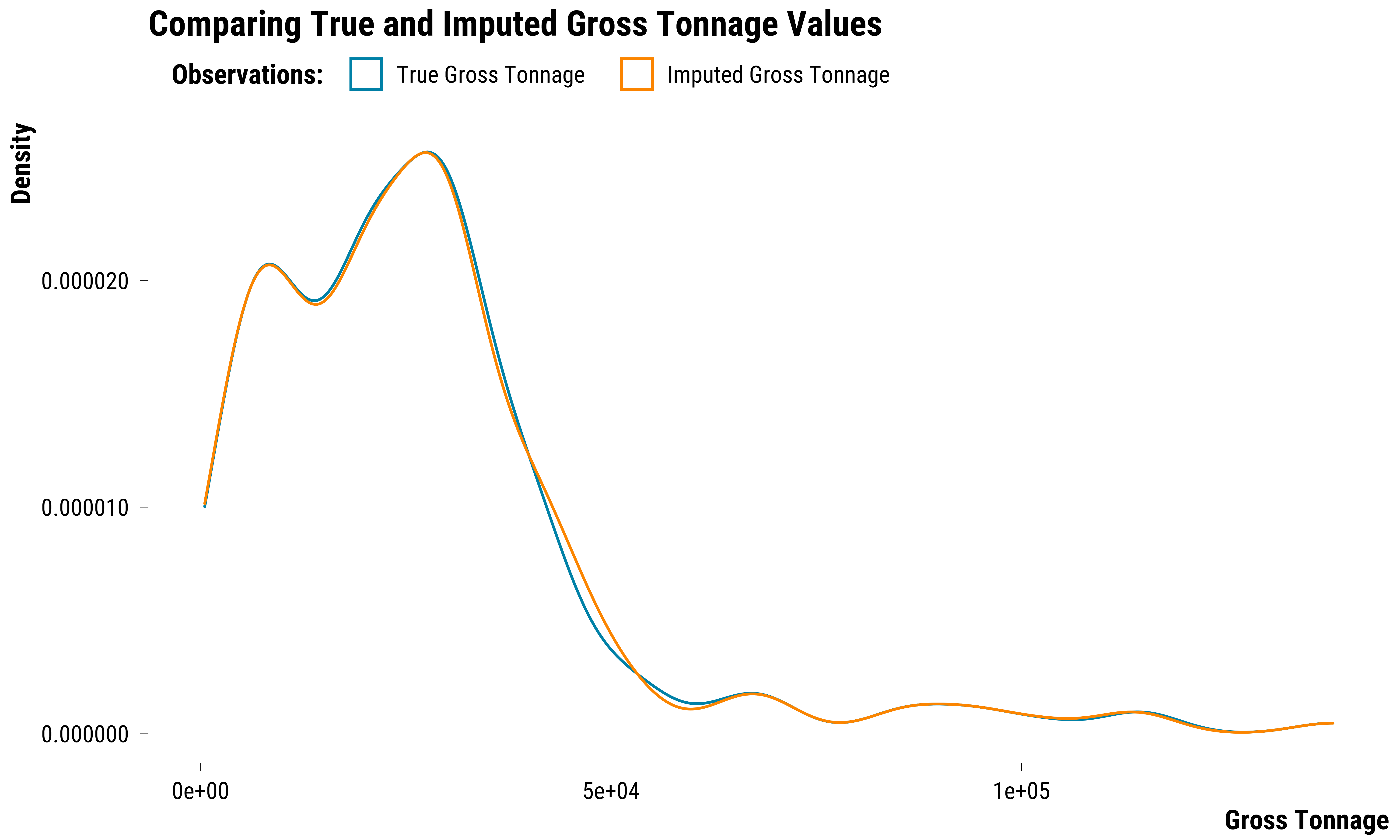
iter 4: ..We can now plot the density distribution of the true values of the gross tonnage observations against the imputed ones:
Please show me the code!
# true gross tonnage values
true_gross_tonnage <- port_data_test %>%
filter(id %in% ids_na) %>%
select(id, gross_tonnage) %>%
rename("True Gross Tonnage" = gross_tonnage)
# imputed gross tonnage values
imputed_gross_tonnage <- port_data_test_imputed %>%
filter(id %in% ids_na) %>%
select(id, gross_tonnage) %>%
rename("Imputed Gross Tonnage" = gross_tonnage)
# joining the true and imputed values together
gross_tonnage_comparison_df <-
left_join(true_gross_tonnage, imputed_gross_tonnage, by = "id")
# plotting the density distributions
gross_tonnage_comparison_df %>%
gather(., key = "variable", value = "value",-id) %>%
ggplot(., aes(x = value, colour = variable)) +
geom_density(alpha = 0.2) +
scale_color_manual(
name = "Observations:",
labels = c("True Gross Tonnage", "Imputed Gross Tonnage"),
values = c(my_blue, my_orange)
) +
ggtitle("Comparing True and Imputed Gross Tonnage Values") +
scale_y_continuous(labels = scales::comma) +
ylab("Density") +
xlab("Gross Tonnage") +
labs(colour = "Observations:") +
theme_tufte()
Below is the table with the true values for gross tonnage and the ones imputed by the algorithm and their difference:
Please show me the code!
# joining the true and imputed values together and computing the difference
gross_tonnage_comparison_df <-
left_join(true_gross_tonnage, imputed_gross_tonnage, by = "id") %>%
mutate(Difference = abs(`True Gross Tonnage` - `Imputed Gross Tonnage`)) %>%
rename("Observation Id" = id)
# print the table
rmarkdown::paged_table(gross_tonnage_comparison_df)
The absolute average difference is 274.6. Given that average gross tonnage value is 2.94014^{4}, this is a relatively small imputation error.
Of course, this is a simple example where the values were erased at random. The imputation algorithm could have more trouble to impute values under different missingness scenarios. We still think it is better to impute our missing observations than dropping them and we should keep in mind that they only represent 0.4 % of the total number of observations.
We now impute the real missing values for the gross tonnage and deadweight tonnage variables:
# replace wrongly recorded gross tonnage and deadweight tonnage observations by missing values
port_data <- port_data %>%
mutate(id = seq(1:41015)) %>%
mutate(
gross_tonnage = ifelse(gross_tonnage < 2, NA, gross_tonnage),
deadweight_tonnage = ifelse(deadweight_tonnage < 2, NA, deadweight_tonnage)
)
# record the index of these variables
ids_na <- port_data %>%
filter(is.na(gross_tonnage)) %>%
select(id) %>%
deframe()
# running the imputation algorithm
port_data <-
missRanger(
port_data,
formula = gross_tonnage + deadweight_tonnage ~ gross_tonnage + deadweight_tonnage + boat_height + boat_max_width,
pmm.k = 3,
num.trees = 50,
seed = 42
)
Missing value imputation by random forests
Variables to impute: gross_tonnage, deadweight_tonnage
Variables used to impute: gross_tonnage, deadweight_tonnage, boat_height, boat_max_width
iter 1: ..
iter 2: ..
iter 3: ..
iter 4: ..
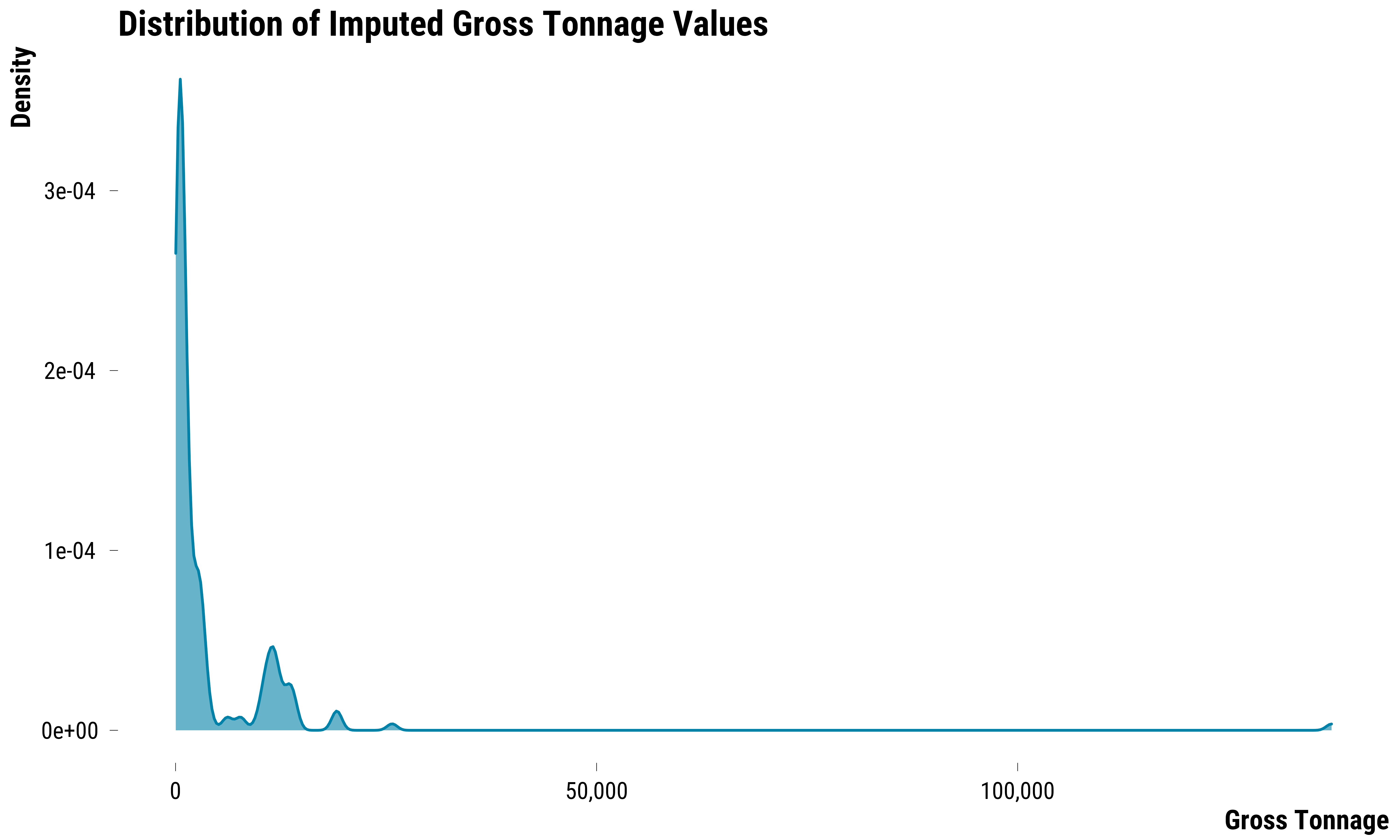
iter 5: ..We plot below the density distribution of the imputed values:
Please show me the code!
And the table for those observations:
Please show me the code!
# print table of imputed observations
rmarkdown::paged_table(port_data %>%
filter(id %in% ids_na))
The gross tonnage summary statistics for imputed missing values are the following ones:
Please show me the code!
port_data %>%
# filter imputed observations
filter(id %in% ids_na) %>%
# select gross tonnage
select(gross_tonnage) %>%
# compute summary statistics
summarise(
"Mean" = round(mean(gross_tonnage, na.rm = TRUE), 1),
"Standard Deviation" = round(sd(gross_tonnage, na.rm = TRUE), 1),
"Minimum" = round(min(gross_tonnage, na.rm = TRUE), 1),
"Maximum" = round(max(gross_tonnage, na.rm = TRUE), 1)
) %>%
# print table
kable(., align = c(rep("c", 4))) %>%
kable_styling(position = "center")
| Mean | Standard Deviation | Minimum | Maximum |
|---|---|---|---|
| 4046.3 | 11067.6 | 24 | 137276 |
Types of boats
Besides gross tonnage, we are also interested in the type of vessels coming to Marseille because:
- the time profile of vessel traffic varies depending on the type of vessel. In particular, it could vary depending on whether the vessel is a cruise or a ferry vessel.
- the division of maritime traffic by vessel type is also important for the analysis of heterogenous treatment effects.
Below we provide the codes used to define the three main categories of vessels docking in Marseille:
- Cruise vessels
- Ferry vessels
- Other types of vessels
#
# we create three dummies for ferry, cruise and other vessel types
#
# we re-classify some roro boats which are actually ferry
port_data <- port_data %>%
mutate(roro_correction_dummy = ifelse(
boat_category == "NAVIRE RO-RO" &
(
holder_name == "KALLISTE" | holder_name == "JEAN NICOLI" |
holder_name == "GIROLATA" |
holder_name == "MONTE D'ORO" |
holder_name == "PAGLIA ORBA" |
holder_name == "PASCAL PAOLI" |
holder_name == "PIANA" |
holder_name == "DENIA CIUTAT CREATIVA"
),
1,
0
))
# dummy for passenger ferry boats: roros that are actually ferry boats, car-ferries, "Ro pax" and "vedettes passagers"
port_data <- port_data %>%
mutate(
ferry_boat = ifelse(
roro_correction_dummy == 1
| boat_category == "CAR-FERRIE"
| boat_category == "ROPAX",
1,
0
)
)
# dummy for passenger cruise boats: boat_category values equal to "PAQUEBOT" PAQUEBOT FLUVIAL" PLAISANCE" "NAV. DE PLAISANCE"
port_data <- port_data %>%
mutate(cruise_boat = ifelse(boat_category == "PAQUEBOT", 1, 0))
# dummy for other boats: all the boats that are not ferry nor cruise boats
port_data <- port_data %>%
mutate(other_boat = ifelse(ferry_boat == 0 &
cruise_boat == 0, 1, 0))
# finally generate gross tonnage variables for each category
port_data <- port_data %>%
mutate(
gross_tonnage_ferry = ferry_boat * gross_tonnage,
gross_tonnage_cruise = cruise_boat * gross_tonnage,
gross_tonnage_other_boat = other_boat * gross_tonnage
)
We have now defined the three types of boats. Below are the proportions of boats belonging to each type:
- 45.4% of boats are ferries
- 11.7% of boats are cruise boats
- NA% of boats are of other types
Final cleaning steps
As final steps, we need to compute the following figures for the total daily “volume” of maritime traffic:
- the daily total entry gross tonnage which is the sum of boats’ gross tonnage entering the port
- the daily total exit gross tonnage which is the sum of boats’ gross tonnage leaving the port
- the daily total gross tonnage which is the sum of the two previous figures
We first transform the entry and exit date variables to keep only the year, the month and the day:
We check that the date variables are correctly coded:
# entry date
summary(port_data$entry_date)
Min. 1st Qu. Median Mean 3rd Qu.
"2008-01-01" "2010-07-21" "2013-05-02" "2013-05-16" "2016-03-11"
Max.
"2018-12-31" # exit date
summary(port_data$exit_date)
Min. 1st Qu. Median Mean 3rd Qu.
"2000-01-01" "2010-07-23" "2013-05-03" "2013-05-18" "2016-03-15"
Max.
"2019-09-12" Overall, the dates seem to be correctly recorded. 43 exit dates belong to the 2019 year which is strange but we will not use them as we restrict our analysis to the 2008-2018 period.
We then compute for each date variable figures on the daily total sum of the gross tonnage variable and the number of boats docking/leaving:
# create figures for the entry date
port_data_entry <- port_data %>%
# compute the following statistics by entry date
group_by(entry_date) %>%
summarise(
n_boats_entry = n(),
n_boats_entry_ferry = sum(ferry_boat),
n_boats_entry_cruise = sum(cruise_boat),
n_boats_entry_other_boat = sum(other_boat),
total_gross_tonnage_entry_ferry = sum(gross_tonnage_ferry),
total_gross_tonnage_entry_cruise = sum(gross_tonnage_cruise),
total_gross_tonnage_entry_other_boat = sum(gross_tonnage_other_boat),
total_gross_tonnage_entry = sum(gross_tonnage)
) %>%
rename(date = entry_date)
# create figures for the exit date
port_data_exit <- port_data %>%
# compute the following statistics by entry date
group_by(exit_date) %>%
summarise(
n_boats_exit = n(),
n_boats_exit_ferry = sum(ferry_boat),
n_boats_exit_cruise = sum(cruise_boat),
n_boats_exit_other_boat = sum(other_boat),
total_gross_tonnage_exit_ferry = sum(gross_tonnage_ferry),
total_gross_tonnage_exit_cruise = sum(gross_tonnage_cruise),
total_gross_tonnage_exit_other_boat = sum(gross_tonnage_other_boat),
total_gross_tonnage_exit = sum(gross_tonnage)
) %>%
rename(date = exit_date)
We then merge these two datasets:
# merge entrey and exist datasets
final_port_data <-
left_join(port_data_entry, port_data_exit, by = "date")
And we compute figures on the sum of the number of boats and the gross tonnage to get the total daily values:
final_port_data <- final_port_data %>%
mutate(
n_boats = n_boats_entry + n_boats_exit,
n_boats_ferry = n_boats_entry_ferry + n_boats_exit_ferry,
n_boats_other_boat = n_boats_entry_other_boat + n_boats_exit_other_boat,
n_boats_cruise = n_boats_entry_cruise + n_boats_exit_cruise,
total_gross_tonnage = total_gross_tonnage_entry + total_gross_tonnage_exit ,
total_gross_tonnage_ferry = total_gross_tonnage_entry_ferry + total_gross_tonnage_exit_ferry,
total_gross_tonnage_other_boat = total_gross_tonnage_entry_other_boat + total_gross_tonnage_exit_other_boat,
total_gross_tonnage_cruise = total_gross_tonnage_entry_cruise + total_gross_tonnage_exit_cruise
)
Below are the newly created data with the date, the total number of boats which docked and left and the total gross tonnage, by flow status (entry/exit) and type of boat:
Please show me the code!
rmarkdown::paged_table(final_port_data)
The summary statistics are the following ones:
Please show me the code!
final_port_data %>%
# drop date
select(-date) %>%
# transform data in long format
pivot_longer(cols = c(n_boats_entry:total_gross_tonnage_cruise), names_to = "Variable", values_to = "value") %>%
# compute the statistics for each variable
group_by(Variable) %>%
summarise("Mean" = round(mean(value, na.rm = TRUE),1),
"Standard Deviation" = round(sd(value, na.rm = TRUE),1),
"Minimum" = round(min(value, na.rm = TRUE),1),
"Maximum" = round(max(value, na.rm = TRUE),1),
"Number of Missing Values" = sum(is.na(value))) %>%
# ungroup data
ungroup() %>%
# sort variable
arrange(Variable) %>%
# print table
kable(., align = c("l", rep("c", 5))) %>%
kable_styling(position = "center")
| Variable | Mean | Standard Deviation | Minimum | Maximum | Number of Missing Values |
|---|---|---|---|---|---|
| n_boats | 20.4 | 6.1 | 3 | 41 | 1 |
| n_boats_cruise | 2.4 | 2.7 | 0 | 18 | 1 |
| n_boats_entry | 10.2 | 3.3 | 1 | 23 | 0 |
| n_boats_entry_cruise | 1.2 | 1.3 | 0 | 9 | 0 |
| n_boats_entry_ferry | 4.6 | 1.9 | 0 | 11 | 0 |
| n_boats_entry_other_boat | 4.4 | 2.3 | 0 | 15 | 0 |
| n_boats_exit | 10.2 | 3.6 | 1 | 24 | 1 |
| n_boats_exit_cruise | 1.2 | 1.3 | 0 | 9 | 1 |
| n_boats_exit_ferry | 4.6 | 1.9 | 0 | 12 | 1 |
| n_boats_exit_other_boat | 4.4 | 2.4 | 0 | 14 | 1 |
| n_boats_ferry | 9.3 | 3.5 | 0 | 23 | 1 |
| n_boats_other_boat | 8.7 | 3.9 | 0 | 23 | 1 |
| total_gross_tonnage | 581249.4 | 260708.1 | 34325 | 1691428 | 1 |
| total_gross_tonnage_cruise | 189417.5 | 231781.8 | 0 | 1245396 | 1 |
| total_gross_tonnage_entry | 290641.4 | 130823.9 | 12189 | 805070 | 0 |
| total_gross_tonnage_entry_cruise | 94694.0 | 116557.9 | 0 | 622698 | 0 |
| total_gross_tonnage_entry_ferry | 139705.2 | 55273.0 | 0 | 342696 | 0 |
| total_gross_tonnage_entry_other_boat | 56242.2 | 34044.5 | 0 | 482367 | 0 |
| total_gross_tonnage_exit | 290559.8 | 137621.3 | 7395 | 962733 | 1 |
| total_gross_tonnage_exit_cruise | 94699.9 | 116066.0 | 0 | 622698 | 1 |
| total_gross_tonnage_exit_ferry | 139706.5 | 54267.5 | 0 | 368501 | 1 |
| total_gross_tonnage_exit_other_boat | 56153.5 | 35800.1 | 0 | 459240 | 1 |
| total_gross_tonnage_ferry | 279431.6 | 101403.6 | 0 | 663733 | 1 |
| total_gross_tonnage_other_boat | 112400.3 | 57243.2 | 0 | 500134 | 1 |
Some variables have only one missing observations. We can print the table of observations with a missing value:
Please show me the code!
final_port_data %>%
filter_all(any_vars(is.na(.))) %>%
rmarkdown::paged_table(.)
Missing values correspond to the 2010-03-23 date where there was a strike of dockers on that day.
The maritime traffic data are now clean !
Air Pollution Data
Pollution data come from AtmoSud, the local air quality agency accredited by the French Ministry of the Environment. Marseille has only two stations monitoring background air pollution: Saint-Louis and Lonchamp stations. Saint Louis station is located 2 to 6 kilometers East or South-East from the port depending on the terminal and monitors nitrogen dioxide (NO2), sulfur dioxide (SO2), and Particulate Matter with a diameter below 2.5 micrometers (PM2.5) and with a diameter between 2.5 and 10 micrometers (PM10). Longchamp station is located 3 to 6 kilometers West or North-West from the port depending on the terminal and monitors NO2, ozone (O3) and PM10.
We gathered daily data from these background monitoring stations for each pollutant. Below is the code to clean the data. We also investigate the presence and distribution of missing values.
- We clean NO2 data with the following code:
# load raw no2 data
data_no2 <-
read.csv(
here::here(
"inputs",
"1.data",
"2.daily_data",
"1.raw_data",
"3.pollution_data",
"raw_marseille_no2_data.csv"
),
sep = ";",
encoding = "UTF-8"
)
data_no2 <- data_no2 %>%
# transform from wide to long
gather(date, mean_no2, X01.01.2008:X31.12.2018) %>%
# select name of the station, date and mean_no2 variables
select(`X.U.FEFF.Station`, date, mean_no2) %>%
# transform back from long to wide
pivot_wider(names_from = `X.U.FEFF.Station`, values_from = mean_no2) %>%
# rename the concentration for each station
rename(mean_no2_sl = "Marseille Saint Louis", mean_no2_l = "Marseille-Longchamp") %>%
# transform the concentrations to numeric
mutate_at(vars(mean_no2_sl:mean_no2_l), ~ as.numeric(.)) %>%
# correct the date variable
mutate(date = str_replace(date, "X", "")) %>%
mutate(date = lubridate::dmy(date)) %>%
# sort by date
arrange(date)
Now that the data are clean, we can look at the summary statistics:
Please show me the code!
data_no2 %>%
select(mean_no2_sl:mean_no2_l) %>%
gather(key = Variable, value = value) %>%
group_by(Variable) %>%
summarise("Mean" = round(mean(value, na.rm = TRUE),1),
"Standard Deviation" = round(sd(value, na.rm = TRUE),1),
"Minimum" = round(min(value, na.rm = TRUE),1),
"Maximum" = round(max(value, na.rm = TRUE),1),
"Number of Missing Values" = sum(is.na(value))) %>%
ungroup() %>%
mutate(Variable = fct_relevel(Variable, "mean_no2_l", "mean_no2_sl")) %>%
arrange(Variable) %>%
mutate(Variable = recode(Variable, mean_no2_l = "Daily Mean NO2 at Longchamp Station (UNIT)",
mean_no2_sl = "Daily Mean NO2 at Saint-Louis Station (UNIT)")) %>%
kable(., align = c("l", rep("c", 5))) %>%
kable_styling(position = "center")
| Variable | Mean | Standard Deviation | Minimum | Maximum | Number of Missing Values |
|---|---|---|---|---|---|
| Daily Mean NO2 at Longchamp Station (UNIT) | 30.0 | 13.4 | 4 | 93 | 120 |
| Daily Mean NO2 at Saint-Louis Station (UNIT) | 36.6 | 16.3 | 3 | 91 | 214 |
3 % of the observations are missing for the Lonchamps stationa and
r, round(sum(is.na(data_no2$mean_no2_sl))/nrow(data_no2)*100,1)
% for the Saint-Louis station. Below is the dataframe for those missing
observations:
Please show me the code!
rmarkdown::paged_table(data_no2 %>% filter(is.na(mean_no2_l) | is.na(mean_no2_sl)))
This table shows that for both stations, missing values often span several consecutive days, suggesting breakdowns in the monitoring system.
- We clean PM10 data with the following code:
# load raw pm10 data
data_pm10 <-
read.csv(
here::here(
"inputs",
"1.data",
"2.daily_data",
"1.raw_data",
"3.pollution_data",
"raw_marseille_pm10_data.csv"
),
sep = ";",
encoding = "UTF-8"
)
data_pm10 <- data_pm10 %>%
# transform from wide to long
gather(date, mean_pm10, X01.01.2008:X31.12.2018) %>%
# select name of the station, date and mean_pm10 variables
select(`X.U.FEFF.Station`, date, mean_pm10) %>%
# transform back from long to wide
pivot_wider(names_from = `X.U.FEFF.Station`, values_from = mean_pm10) %>%
# rename the concentration for each station
rename(mean_pm10_sl = "Marseille Saint Louis", mean_pm10_l = "Marseille-Longchamp") %>%
# transform the concentrations to numeric
mutate_at(vars(mean_pm10_sl:mean_pm10_l), ~ as.numeric(.)) %>%
# correct the date variable
mutate(date = str_replace(date, "X", "")) %>%
mutate(date = lubridate::dmy(date)) %>%
# sort by date
arrange(date)
Now that the data are clean, we can look at the summary statistics:
Please show me the code!
data_pm10 %>%
select(mean_pm10_sl:mean_pm10_l) %>%
gather(key = Variable, value = value) %>%
group_by(Variable) %>%
summarise("Mean" = round(mean(value, na.rm = TRUE),1),
"Standard Deviation" = round(sd(value, na.rm = TRUE),1),
"Minimum" = round(min(value, na.rm = TRUE),1),
"Maximum" = round(max(value, na.rm = TRUE),1),
"Number of Missing Values" = sum(is.na(value))) %>%
ungroup() %>%
mutate(Variable = fct_relevel(Variable, "mean_pm10_l", "mean_pm10_sl")) %>%
arrange(Variable) %>%
mutate(Variable = recode(Variable, mean_pm10_l = "Daily Mean PM10 at Longchamp Station (UNIT)",
mean_pm10_sl = "Daily Mean PM10 at Saint-Louis Station (UNIT)")) %>%
kable(., align = c("l", rep("c", 5))) %>%
kable_styling(position = "center")
| Variable | Mean | Standard Deviation | Minimum | Maximum | Number of Missing Values |
|---|---|---|---|---|---|
| Daily Mean PM10 at Longchamp Station (UNIT) | 27.0 | 10.8 | 5 | 114 | 250 |
| Daily Mean PM10 at Saint-Louis Station (UNIT) | 30.7 | 15.3 | 3 | 176 | 410 |
6.2 % of the observations are missing for the Lonchamp station and
r, round(sum(is.na(data_pm10$mean_pm10_sl))/nrow(data_pm10)*100,1)
% for the Saint-Louis station. Below is the dataframe for those missing
observations:
Please show me the code!
rmarkdown::paged_table(data_pm10 %>% filter(is.na(mean_pm10_l) | is.na(mean_pm10_sl)))
Again, this table shows that for both stations, missing values span often over several consecutive days which points out that the station must have broken down.
- We clean PM25 data with the following code:
# load raw pm25 data
data_pm25 <- read.csv(here::here("inputs", "1.data", "2.daily_data", "1.raw_data", "3.pollution_data", "raw_marseille_pm25_data.csv"), sep=";", encoding = "UTF-8")
data_pm25 <- data_pm25 %>%
# transform from wide to long
gather(date, mean_pm25, X01.01.2008:X31.12.2018) %>%
# select name of the station, date and mean_pm25 variables
select(`X.U.FEFF.Station`, date, mean_pm25) %>%
# transform back from long to wide
pivot_wider(names_from = `X.U.FEFF.Station`, values_from = mean_pm25) %>%
# rename the concentration for each station
rename(mean_pm25_l = "Marseille-Longchamp") %>%
# transform the concentrations to numeric
mutate_at(vars(mean_pm25_l), ~ as.numeric(.)) %>%
# correct the date variable
mutate(date = str_replace(date, "X", "")) %>%
mutate(date = lubridate::dmy(date)) %>%
# sort by date
arrange(date)
Now that the data are clean, we can look at the summary statistics:
Please show me the code!
data_pm25 %>%
select(mean_pm25_l) %>%
gather(key = Variable, value = value) %>%
group_by(Variable) %>%
summarise("Mean" = round(mean(value, na.rm = TRUE),1),
"Standard Deviation" = round(sd(value, na.rm = TRUE),1),
"Minimum" = round(min(value, na.rm = TRUE),1),
"Maximum" = round(max(value, na.rm = TRUE),1),
"Number of Missing Values" = sum(is.na(value))) %>%
ungroup() %>%
mutate(Variable = fct_relevel(Variable, "mean_pm25_l")) %>%
arrange(Variable) %>%
mutate(Variable = recode(Variable, mean_pm25_l = "Daily Mean PM25 at Longchamp Station (UNIT)")) %>%
kable(., align = c("l", rep("c", 5))) %>%
kable_styling(position = "center")
| Variable | Mean | Standard Deviation | Minimum | Maximum | Number of Missing Values |
|---|---|---|---|---|---|
| Daily Mean PM25 at Longchamp Station (UNIT) | 15.4 | 8.5 | 0 | 77 | 436 |
10.9 % of the observations are missing for the Lonchamps station. Below is the dataframe for those missing observations:
Please show me the code!
rmarkdown::paged_table(data_pm25 %>% filter(is.na(mean_pm25_l)))
Again, this table shows that for the measuring station, missing values span often over several consecutive days which points out that the station must have broken down.
- We clean SO2 data with the following code:
# load raw so2 data
data_so2 <- read.csv(here::here("inputs", "1.data", "2.daily_data", "1.raw_data", "3.pollution_data", "raw_marseille_so2_data.csv"), sep=";", encoding = "UTF-8")
data_so2 <- data_so2 %>%
# transform from wide to long
gather(date, mean_so2, X01.01.2008:X31.12.2018) %>%
# select name of the station, date and mean_so2 variables
select(`X.U.FEFF.Station`, date, mean_so2) %>%
# transform back from long to wide
pivot_wider(names_from = `X.U.FEFF.Station`, values_from = mean_so2) %>%
# rename the concentration for each station
rename(mean_so2_l = "Marseille-Longchamp") %>%
# transform the concentrations to numeric
mutate_at(vars(mean_so2_l), ~ as.numeric(.)) %>%
# correct the date variable
mutate(date = str_replace(date, "X", "")) %>%
mutate(date = lubridate::dmy(date)) %>%
# sort by date
arrange(date)
Now that the data are clean, we can look at the summary statistics:
Please show me the code!
data_so2 %>%
select(mean_so2_l) %>%
gather(key = Variable, value = value) %>%
group_by(Variable) %>%
summarise("Mean" = round(mean(value, na.rm = TRUE),1),
"Standard Deviation" = round(sd(value, na.rm = TRUE),1),
"Minimum" = round(min(value, na.rm = TRUE),1),
"Maximum" = round(max(value, na.rm = TRUE),1),
"Number of Missing Values" = sum(is.na(value))) %>%
ungroup() %>%
mutate(Variable = fct_relevel(Variable, "mean_so2_l")) %>%
arrange(Variable) %>%
mutate(Variable = recode(Variable, mean_so2_l = "Daily Mean SO2 at Longchamp Station (UNIT)")) %>%
kable(., align = c("l", rep("c", 5))) %>%
kable_styling(position = "center")
| Variable | Mean | Standard Deviation | Minimum | Maximum | Number of Missing Values |
|---|---|---|---|---|---|
| Daily Mean SO2 at Longchamp Station (UNIT) | 2.3 | 2.5 | 0 | 32 | 201 |
5 % of the observations are missing for the Lonchamps station. Below is the dataframe for those missing observations:
Please show me the code!
rmarkdown::paged_table(data_so2 %>% filter(is.na(mean_so2_l)))
- We clean O3 data with the following code:
# load raw o3 data
data_o3 <- read.csv(here::here("inputs", "1.data", "2.daily_data", "1.raw_data", "3.pollution_data", "raw_marseille_o3_data.csv"), sep=";", encoding = "UTF-8")
data_o3 <- data_o3 %>%
# transform from wide to long
gather(date, mean_o3, X01.01.2008:X31.12.2018) %>%
# select name of the station, date and mean_o3 variables
select(`X.U.FEFF.Station`, date, mean_o3) %>%
# transform back from long to wide
pivot_wider(names_from = `X.U.FEFF.Station`, values_from = mean_o3) %>%
# rename the concentration for each station
rename(mean_o3_l = "Marseille-Longchamp") %>%
# transform the concentrations to numeric
mutate_at(vars(mean_o3_l), ~ as.numeric(.)) %>%
# correct the date variable
mutate(date = str_replace(date, "X", "")) %>%
mutate(date = lubridate::dmy(date)) %>%
# sort by date
arrange(date)
Now that the data are clean, we can look at the summary statistics:
Please show me the code!
data_o3 %>%
select(mean_o3_l) %>%
gather(key = Variable, value = value) %>%
group_by(Variable) %>%
summarise("Mean" = round(mean(value, na.rm = TRUE),1),
"Standard Deviation" = round(sd(value, na.rm = TRUE),1),
"Minimum" = round(min(value, na.rm = TRUE),1),
"Maximum" = round(max(value, na.rm = TRUE),1),
"Number of Missing Values" = sum(is.na(value))) %>%
ungroup() %>%
mutate(Variable = fct_relevel(Variable, "mean_o3_l")) %>%
arrange(Variable) %>%
mutate(Variable = recode(Variable, mean_o3_l = "Daily Mean o3 at Longchamp Station (UNIT)")) %>%
kable(., align = c("l", rep("c", 5))) %>%
kable_styling(position = "center")
| Variable | Mean | Standard Deviation | Minimum | Maximum | Number of Missing Values |
|---|---|---|---|---|---|
| Daily Mean o3 at Longchamp Station (UNIT) | 53.8 | 23 | 2 | 121 | 150 |
3.7 % of the observations are missing for the Lonchamps station. Below is the dataframe for those missing observations:
Please show me the code!
rmarkdown::paged_table(data_o3 %>% filter(is.na(mean_o3_l)))
Finally, we merge the pollutants data together:
# merging all pollutants files together
marseille_pollutants <- data_no2 %>%
full_join(data_pm10, by = "date") %>%
full_join(data_pm25, by = "date") %>%
full_join(data_so2, by = "date") %>%
full_join(data_o3, by = "date")
We save the marseille_pollutants data, which are not imputed, because we will use them to see how our analysis on the matched data differs between imputed and non-imputed pollutant concentrations:
Below is the dataframe of pollution variables:
Please show me the code!
rmarkdown::paged_table(marseille_pollutants)
The pollutants data are now ready to be matched with the other datasets.
Weather Data
We obtained daily weather data from Meteo-France, the French national meteorological service. We used data from Marseille airport’s weather station, the only weather station located near Marseille (about 25 km away). We extracted observations on rainfall duration (min), rainfall height (mm), average temperature (°C) and humidity (%), wind speed (m/s) and the direction from which the wind blows (measured on a 360 degrees compass rose):
# read the data and rename the variables
weather_data <-
read.csv(
here::here(
"inputs",
"1.data",
"2.daily_data",
"1.raw_data",
"4.weather_data",
"raw_data_weather_marseille.txt"
),
header = TRUE,
sep = ";",
stringsAsFactors = FALSE,
dec = ","
) %>%
rename(
"date" = "DATE",
"rainfall_height" = "RR",
"rainfall_duration" = "DRR",
"temperature_minimum" = "TN",
"temperature_maximun" = "TX",
"temperature_average" = "TM",
"humidity_average" = "UM",
"wind_speed" = "FFM",
"wind_direction" = "DXY"
) %>%
select(-POSTE)
# convert date variable in date format
weather_data <- weather_data %>%
mutate(date = lubridate::ymd(weather_data$date))
Below is the dataframe of the weather variables:
Please show me the code!
rmarkdown::paged_table(weather_data)
Below are the summary statistics for continuous weather variables:
Please show me the code!
rmarkdown::paged_table(weather_data)
Please show me the code!
weather_data %>%
select(rainfall_height:wind_speed, humidity_average) %>%
gather(key = Variable, value = value) %>%
group_by(Variable) %>%
summarise("Mean" = round(mean(value, na.rm = TRUE),1),
"Standard Deviation" = round(sd(value, na.rm = TRUE),1),
"Minimum" = round(min(value, na.rm = TRUE),1),
"Maximum" = round(max(value, na.rm = TRUE),1),
"Number of Missing Values" = sum(is.na(value))) %>%
ungroup() %>%
mutate(Variable = fct_relevel(Variable, "rainfall_height", "rainfall_duration", "temperature_minimum",
"temperature_maximun", "temperature_average", "humidity_average",
"wind_speed", "wind_direction")) %>%
arrange(Variable) %>%
mutate(Variable = recode(Variable, rainfall_height = "Rainfall Height (cm)",
rainfall_duration = "Rainfall Duration (min)",
temperature_minimum = "Minimum Temperature (°C)",
temperature_average = "Average Temperature (°C)",
temperature_maximum = "Maximum Temperature (°C)",
humidity_average = "Average Humidity (%)",
wind_speed = "Wind Speed (m/s)")) %>%
kable(., align = c("l", rep("c", 5))) %>%
kable_styling(position = "center")
| Variable | Mean | Standard Deviation | Minimum | Maximum | Number of Missing Values |
|---|---|---|---|---|---|
| Rainfall Height (cm) | 1.6 | 5.9 | 0.0 | 104.2 | 0 |
| Rainfall Duration (min) | 63.1 | 165.5 | 0.0 | 1440.0 | 60 |
| Minimum Temperature (°C) | 11.2 | 6.7 | -9.5 | 28.0 | 0 |
| temperature_maximun | 21.0 | 7.6 | -1.0 | 39.2 | 0 |
| Average Temperature (°C) | 15.9 | 7.0 | -3.5 | 31.3 | 0 |
| Average Humidity (%) | 65.2 | 12.4 | 30.0 | 96.0 | 1 |
| Wind Speed (m/s) | 4.7 | 2.8 | 0.4 | 17.8 | 0 |
We can see from these tables that we have very few missing variables.
The weather data are now ready to be merged with the other datasets.
Road traffic data (2011-2016 period)
We import road traffic data at the daily level for the 2011-2016 period. We several measurements of road traffic which were averaged at the city-level over 6 stations:
Below are the summary statistics for the daily flow of vehicles:
Please show me the code!
road_traffic_data %>%
pivot_longer(cols = -c(date), names_to = "Road Traffic Measure", values_to = "value") %>%
group_by(`Road Traffic Measure`) %>%
summarise(
"Mean" = round(mean(value, na.rm = TRUE), 0),
"Standard Deviation" = round(sd(value, na.rm = TRUE), 0),
"Minimum" = round(min(value, na.rm = TRUE), 0),
"Maximum" = round(max(value, na.rm = TRUE), 0),
"Number of Missing Values" = sum(is.na(value))
) %>%
kable(., align = c("l", rep("c", 5))) %>%
kable_styling(position = "center")
| Road Traffic Measure | Mean | Standard Deviation | Minimum | Maximum | Number of Missing Values |
|---|---|---|---|---|---|
| road_occupancy_rate | 11 | 3 | 0 | 22 | 1 |
| road_traffic_flow_all | 2163 | 382 | 5 | 4392 | 1 |
| road_traffic_flow_trucks | 30 | 15 | 0 | 61 | 1 |
| road_traffic_speed_all | 90 | 5 | 73 | 106 | 1 |
| road_traffic_speed_trucks | 80 | 4 | 67 | 110 | 4 |
Calendar Indicators, Bank Days and Holidays Data
First, we create a dataframe with the date variable, the year, the season, the month, the weekend dummy and the day of the week:
# create a dataframe with the date variable
dates_data <-
tibble(date = seq.Date(
from = as.Date("2008-01-01"),
to = as.Date("2018-12-31"),
by = "day"
))
# create year, month and day of the week indicators
dates_data <- dates_data %>%
mutate(
year = lubridate::year(date),
season = lubridate::quarter(date),
month = lubridate::month(date, label = TRUE, abbr = FALSE),
weekday = lubridate::wday(date, label = TRUE, abbr = FALSE)
)
# reorder day of the week levels
dates_data <- dates_data %>%
mutate(weekday = ordered(
weekday,
levels = c(
"Monday",
"Tuesday",
"Wednesday",
"Thursday",
"Friday",
"Saturday",
"Sunday"
)
))
# create a dummy for the weekend
dates_data <- dates_data %>%
mutate(weekend = ifelse(weekday == "Saturday" |
weekday == "Sunday", 1, 0))
Then, we load two datasets on holidays and bank days indicators:
# cleaning holidays data
data_holidays <-
read.csv(
here::here(
"inputs",
"1.data",
"2.daily_data",
"1.raw_data",
"5.bank_days_holidays_data",
"data_holidays.csv"
),
stringsAsFactors = FALSE,
encoding = "UTF-8"
) %>%
select(date, vacances_zone_b, nom_vacances) %>%
rename(holidays_dummy = vacances_zone_b, holidays_name = nom_vacances) %>%
mutate(holidays_dummy = ifelse(holidays_dummy == "True", 1, 0)) %>%
mutate(date = lubridate::ymd(date)) %>%
filter(date >= "2008-01-01" & date < "2019-01-01")
# cleaning bank days data
data_bank_days <-
read.csv(
here::here(
"inputs",
"1.data",
"2.daily_data",
"1.raw_data",
"5.bank_days_holidays_data",
"data_bank_days.csv"
),
stringsAsFactors = FALSE,
encoding = "UTF-8"
) %>%
rename(bank_day_dummy = est_jour_ferie, name_bank_day = nom_jour_ferie) %>%
mutate(bank_day_dummy = ifelse(bank_day_dummy == "True", 1, 0)) %>%
mutate(date = lubridate::ymd(date)) %>%
filter(date >= "2008-01-01" & date < "2019-01-01")
We merge the three datasets together:
# merge the three datasets together
dates_data <- left_join(dates_data, data_holidays, by = "date") %>%
left_join(., data_bank_days, by = "date")
Below is the dataframe for the time indicators:
Please show me the code!
rmarkdown::paged_table(dates_data)
Merging all Data
We finally need to merge all the datasets together.
Merging calendar, pollution and weather data
We first merge the date, pollution and weather data together:
# we first merge calendar data and pollution data
data <- left_join(dates_data, marseille_pollutants, by = "date") %>%
# then we merge the two datasets with the weather data
left_join(., weather_data, by = "date")
Merging with maritime traffic and road traffic data
We merge the data with the two daily-level remaining datasets on maritime and road traffic:
# merge with maritime traffic data
data <- left_join(data, final_port_data, by = "date") %>%
# merge with maritime traffic data
left_join(., road_traffic_data, by = "date")
Imputing missing values for air pollution and weather variables
We finally impute missing values for air pollution and weather variables.
Simulation Exercice
Before carrying out the imputation procedure, we provide evidence that the missRanger package works well in this framework. Similar to our test in the boat data section, we carry out a simulation to show that imputed values are close to real values. We start by creating the data_test where we drop all rows that contain at least a missing value for a selected subset of variables.
# create data_test
data_test <- data %>%
# select relevant variables for the imputation exercise
select(
# calendar variable
date,
year,
month,
weekday,
holidays_dummy,
bank_day_dummy,
# pollutants
mean_no2_sl:mean_o3_l,
# weather variables
rainfall_height:humidity_average,
# vessel and road traffic variables
total_gross_tonnage,
road_traffic_flow_all,
road_occupancy_rate
) %>%
# drop rows with at least a missing value
drop_na() %>%
# create an index
mutate(id = seq(1:n()))
To mimick measuring stations that break down, we are going to erase values for observations that belong to four weeks selected at random. However, we are are not going to erase values for all variables that belong to these weeks. Concomitant missingness of all variables does not happen in our data. We choose to erase values for NO2 and PM2.5 pollutants measured at Longchamp station. NO2 is also measured at Saint-Louis station so the algorithm might be able to use its records to impute concentrations at Longchamp station. PM2.5 is however only measured at Longchamp station so the algorithm will not be able to use concentrations measured at the time from other stations. Below is the code to create missing values:
# weeks whose observations should be erased
weeks_selected <- sample(seq(1:52), 4)
# create the week variables
data_test <- data_test %>%
mutate(week = lubridate::week(date))
# create data_test_na where we erase values for selected weeks
data_test_na <- data_test %>%
# select relevant weeks
filter(week %in% weeks_selected) %>%
# erase values for those observations
mutate_at(vars(mean_no2_l, mean_pm25_l), ~ . == NA)
# bind data_test without the missing values with data_test_na
data_test_na <-
bind_rows((data_test %>% filter(!(
week %in% weeks_selected
))), data_test_na)
We impute the missing values using the missRanger algorithm. We
impute mean_no2_l and mean_pm25_l
concentrations using all variables but the date, the id of the row and
the minimum and maximum temperature as they did not seem to help better
predict missing values. We take as parameters 100 trees and 10 for the
pmm.k parameter:
# running the imputation algorithm
data_test_imputed <-
missRanger::missRanger(
data_test_na,
mean_no2_l + mean_pm25_l ~ . - date - id - temperature_minimum - temperature_maximum,
pmm.k = 10,
num.trees = 100,
seed = 42
)
Missing value imputation by random forests
Variables to impute: mean_no2_l, mean_pm25_l
Variables used to impute: year, month, weekday, holidays_dummy, bank_day_dummy, mean_no2_sl, mean_no2_l, mean_pm10_sl, mean_pm10_l, mean_pm25_l, mean_so2_l, mean_o3_l, rainfall_height, rainfall_duration, temperature_maximun, temperature_average, wind_speed, wind_direction, humidity_average, total_gross_tonnage, road_traffic_flow_all, road_occupancy_rate, week
iter 1: ..
iter 2: ..
iter 3: ..
iter 4: ..
iter 5: ..We can check that missing NO2 values were correctly imputed:
Please show me the code!
# true no2 at Longchamp station
true_no2_l <- data_test %>%
filter(week %in% weeks_selected) %>%
select(id, mean_no2_l) %>%
rename("True NO2 at Longchamp" = mean_no2_l)
# imputed no2 at saint-louis station
imputed_no2_l <- data_test_imputed %>%
filter(week %in% weeks_selected) %>%
select(id, mean_no2_l) %>%
rename("Imputed NO2 at Longchamp" = mean_no2_l)
# combining true and imputed no2 values together
no2_comparison_df <-
left_join(true_no2_l, imputed_no2_l, by = "id")
# plotting density distributions
no2_comparison_df %>%
gather(., key = "variable", value = "value",-id) %>%
ggplot(., aes(x = value, colour = variable)) +
geom_density(alpha = 0.2) +
scale_color_manual(
name = "Observations:",
labels = c("True NO2 at Longchamp", "Imputed NO2 at Longchamp"),
values = c(my_blue, my_orange)
) +
scale_y_continuous(labels = scales::comma) +
ylab("Density") +
xlab("Daily Mean NO2") +
labs(colour = "Observations:") +
theme_tufte()
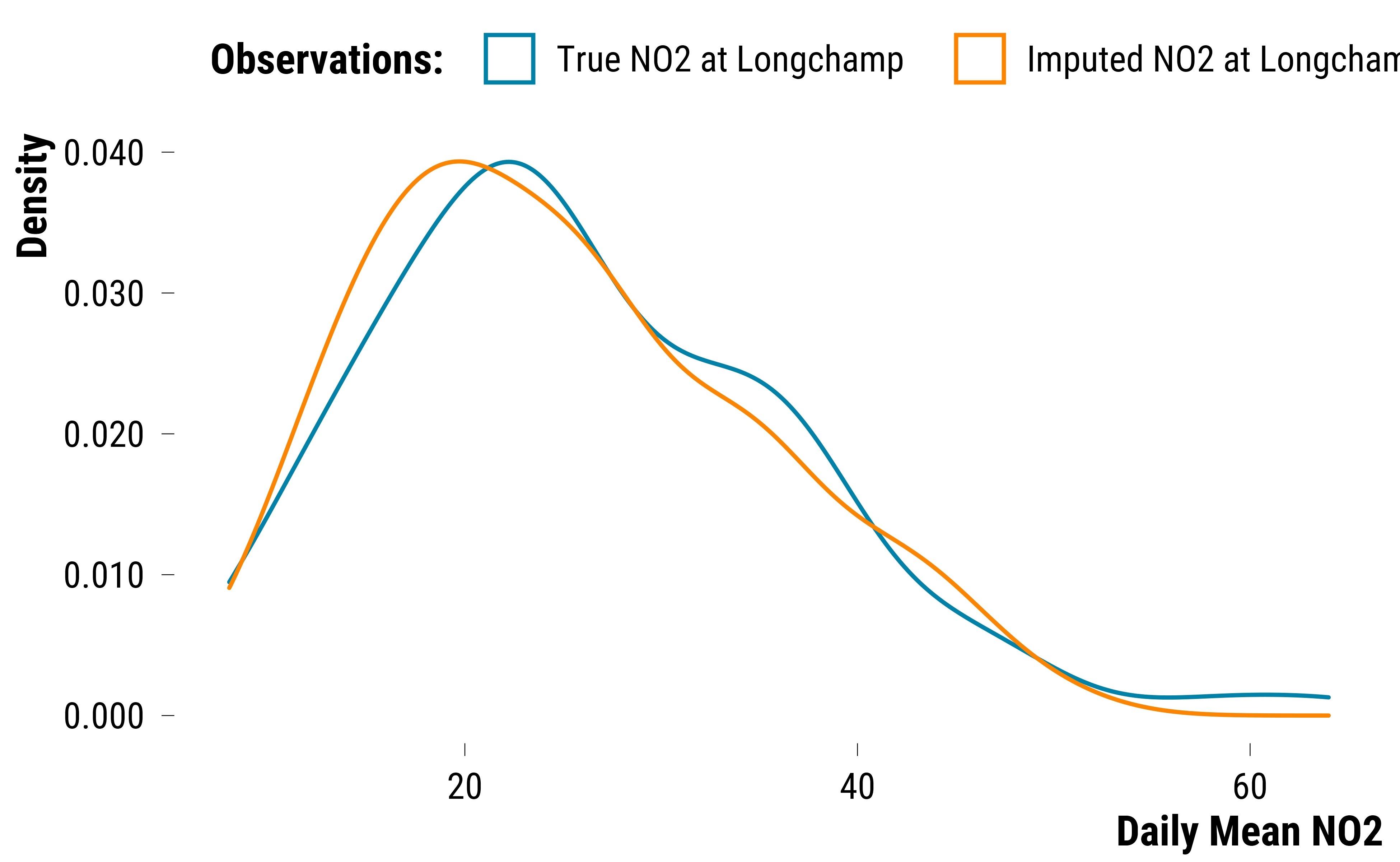
The overlap of the two densities is not perfect but seems decent. We show below the table with the true and imputed values for NO2:
Please show me the code!
# joining the true and imputed values together and computing the difference
no2_comparison_df <-
left_join(true_no2_l, imputed_no2_l, by = "id") %>%
mutate(Difference = abs(`True NO2 at Longchamp` - `Imputed NO2 at Longchamp`)) %>%
rename("Observation Id" = id)
rmarkdown::paged_table(no2_comparison_df)
The absolute average difference is 3.7. Given that the daily NO2 average is 30, we think it is a fair imputation result. We plot below the distribution of the true PM2.5 concentrations and the ones imputed:
Please show me the code!
# true pm2.5 at Longchamp station
true_pm25_l <- data_test %>%
filter(week %in% weeks_selected) %>%
select(id, mean_pm25_l) %>%
rename("True PM2.5 at Longchamp" = mean_pm25_l)
# imputed pm2.5 atat Longchamp station
imputed_pm25_l <- data_test_imputed %>%
filter(week %in% weeks_selected) %>%
select(id, mean_pm25_l) %>%
rename("Imputed PM2.5 at Longchamp" = mean_pm25_l)
# combining true and imputed pm2.5 values together
pm25_comparison_df <-
left_join(true_pm25_l, imputed_pm25_l, by = "id")
# plotting density distributions
pm25_comparison_df %>%
gather(., key = "variable", value = "value",-id) %>%
ggplot(., aes(x = value, colour = variable)) +
geom_density(alpha = 0.2) +
scale_color_manual(
name = "Observations:",
labels = c("True PM2.5 at Longchamp", "Imputed PM2.5 at Longchamp"),
values = c(my_blue, my_orange)
) +
scale_y_continuous(labels = scales::comma) +
ylab("Density") +
xlab("Daily Mean PM2.5") +
labs(colour = "Observations:") +
theme_tufte() +
theme(
legend.position = "top",
legend.justification = "left",
legend.direction = "horizontal"
)
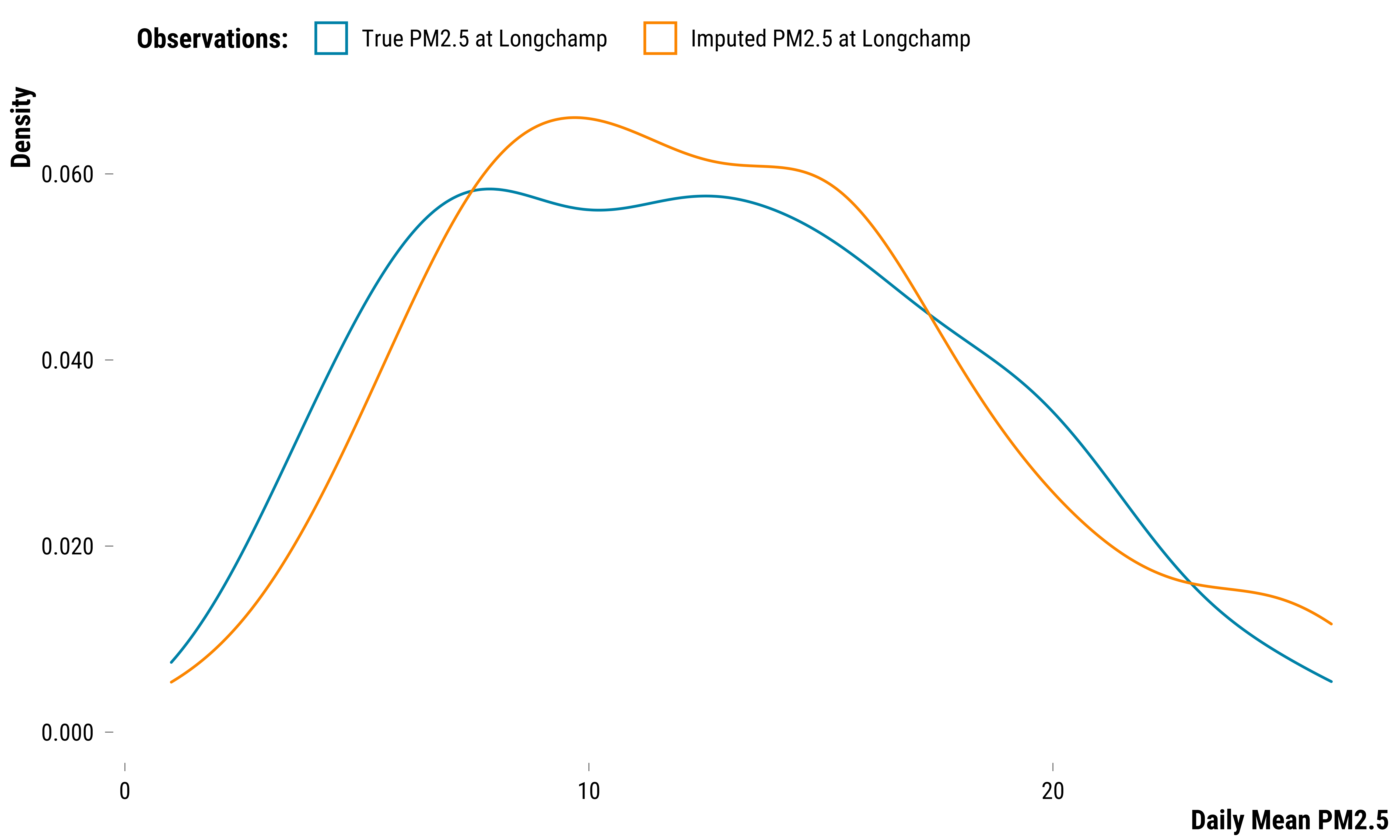
The overlap of the two densities is again not perfect but seems decent. We show below the table of the true and imputed values for each observation and the absolute difference:
Please show me the code!
# joining the true and imputed values together and computing the difference
pm25_comparison_df <-
left_join(true_pm25_l, imputed_pm25_l, by = "id") %>%
mutate(Difference = abs(`True PM2.5 at Longchamp` - `Imputed PM2.5 at Longchamp`)) %>%
rename("Observation Id" = id)
rmarkdown::paged_table(pm25_comparison_df)
The absolute average difference is 2.6. Given that the daily average of PM2.5 is 15.4, this is again a fair imputation error but it happens that the imputation error can be large for several days.
It seems therefore that the imputation algorithm works fine in this small simulation exercise. Yet, we should keep in mind that if many weather variables or co-pollutants were happened to be missing at the same time of a monitoring station’s failure, the algorithm would have troubles correctly predicting its values.
Imputation Procedure
We finally impute the real missing values for the data:
data <- missRanger::missRanger(
data,
# variables to impute
mean_no2_sl + mean_no2_l + mean_pm10_sl + mean_pm10_l + mean_pm25_l + mean_so2_l + mean_o3_l + rainfall_height + rainfall_duration + temperature_average + wind_speed + wind_direction + humidity_average ~
# variables used for the imputation
mean_no2_sl + mean_no2_l + mean_pm10_sl + mean_pm10_l + mean_pm25_l + mean_so2_l + mean_o3_l + rainfall_height + rainfall_duration + temperature_average + wind_speed + wind_direction + humidity_average + total_gross_tonnage + road_traffic_flow_all + road_occupancy_rate + weekday + holidays_dummy + bank_day_dummy + month + year,
pmm.k = 10,
num.trees = 100,
seed = 42
)
Missing value imputation by random forests
Variables to impute: mean_no2_sl, mean_no2_l, mean_pm10_sl, mean_pm10_l, mean_pm25_l, mean_so2_l, mean_o3_l, rainfall_duration, wind_direction, humidity_average
Variables used to impute: mean_no2_sl, mean_no2_l, mean_pm10_sl, mean_pm10_l, mean_pm25_l, mean_so2_l, mean_o3_l, rainfall_height, rainfall_duration, temperature_average, wind_speed, wind_direction, humidity_average, weekday, holidays_dummy, bank_day_dummy, month, year
iter 1: ..........
iter 2: ..........
iter 3: ..........
iter 4: ..........Final Cleaning Steps
Creating Rainfall Dummy and Wind Direction Categories
We create a dummy for the rainfall_height variable to
know if for a given day it rained:
# create u and v components of the wind vector
data <- data %>%
mutate(rainfall_height_dummy = ifelse(rainfall_height > 0, 1, 0))
We can also sort the wind direction into four main directions (North-East, South-East, South-West, North-West):
# create u and v components of the wind vector
data <- data %>%
mutate(
wind_direction_categories = cut(
wind_direction,
breaks = seq(0, 360, by = 90),
include.lowest = TRUE
) %>%
recode(
.,
"[0,90]" = "North-East",
"(90,180]" = "South-East",
"(180,270]" = "South-West",
"(270,360]" = "North-West"
)
)
We also also sort the wind direction into two main directions (East and West) as they are two broad directions that could matter to bring or chase pollution emitted by vessels:
Saving the Data
We reorder the variables:
data <- data %>%
select(# calendar indicators
date:name_bank_day,
# pollutants
mean_no2_sl:mean_o3_l,
# weather parameters
rainfall_height:wind_direction_east_west,
# maritime traffic variables
total_gross_tonnage,
n_boats_cruise, n_boats_ferry, n_boats_entry_other_boat,
total_gross_tonnage_cruise, total_gross_tonnage_ferry, total_gross_tonnage_other_boat,
n_boats_entry, n_boats_entry_cruise, n_boats_entry_ferry, n_boats_entry_other_boat,
n_boats_exit, n_boats_exit_cruise, n_boats_exit_ferry, n_boats_exit_other_boat,
total_gross_tonnage_entry, total_gross_tonnage_entry_cruise, total_gross_tonnage_entry_ferry, total_gross_tonnage_entry_other_boat,
total_gross_tonnage_exit, total_gross_tonnage_exit_cruise, total_gross_tonnage_exit_ferry, total_gross_tonnage_exit_other_boat,
# road traffic variable
road_traffic_flow_all, road_occupancy_rate)
The data are now ready to be analyzed. Below is the table of the dataframe:
Please show me the code!
rmarkdown::paged_table(data)
We save the data in the 1.data/2.data_for_analysis folder: