In this document, we carry out an exploratory data analysis to investigate the parallel evolution of road traffic and nitrogen dioxide (NO $_{2}$ ) concentrations in Marseille. We focus on NO $_{2}$ as it is locally emitted by cars. We carry out a simple analysis where compare the concentration of NO $_{2}$ between weekdays and weekends as road traffic tends to decrease on Saturday and Sunday. The weekend/weedays contrast can be seen as a form of arbitrary variation in road traffic. We do not check the effects on other pollutants because they are less emitted locally.

In the following sections, we proceed as follows:

We show that road traffic is indeed lower on weekends and that NO $_{2}$ concentrations fall at the end of the week.
We check that weather covariates are balanced across weekdays and weekends.
We compute the difference in NO $_{2}$ concentrations between weekdays and weekends.

Should you have any questions, need help to reproduce the analysis or find coding errors, please do not hesitate to contact us at leo.zabrocki@gmail.com and marion.leroutier@hhs.se.

Required Packages

We load the following packages:

# load required packages
library(knitr) # for creating the R Markdown document
library(here) # for files paths organization
library(tidyverse) # for data manipulation and visualization
library(kableExtra) # for table formatting
library(Cairo) # for printing custom police of graphs

We load our custom ggplot2 theme for graphs:

# load ggplot custom theme
source(here::here("inputs",
                  "2.functions",
                  "script_theme_tufte.R"))
# define nice colors
my_blue <- "#0081a7"
my_orange <- "#fb8500"

Data Loading and Formatting

First, we load the daily data:

# load data
data <-
  readRDS(
    here(
      "inputs",
      "1.data",
      "2.daily_data",
      "2.data_for_analysis",
      "0.main_data",
      "data_for_analysis_daily.RDS"
    )
  )

We select relevant variables for our analysis:

data <- data %>%
  select(
    # date variable
    "date",
    # pollutants
    "mean_no2_l",
    "mean_no2_sl",
    # maritime traffic variables
    "total_gross_tonnage_cruise",
    # weather parameters
    "temperature_average",
    "rainfall_height_dummy",
    "humidity_average",
    "wind_speed",
    "wind_direction_categories",
    # road traffic variables
    "road_traffic_flow_all",
    "road_occupancy_rate",
    # calendar indicators
    "weekday",
    "weekend",
    "holidays_dummy",
    "bank_day_dummy",
    "month",
    "year"
  )

Exploratory Data Analysis

Road Traffic Variation by Day of the Week

We explore the patterns of road traffic. It is important to keep in mind that:

We only use six stations in Marseille to create aggregated measures of traffic.
Some stations have an important number of missing values.
Data are available only from 2011-01-01 to 2016-10-02.

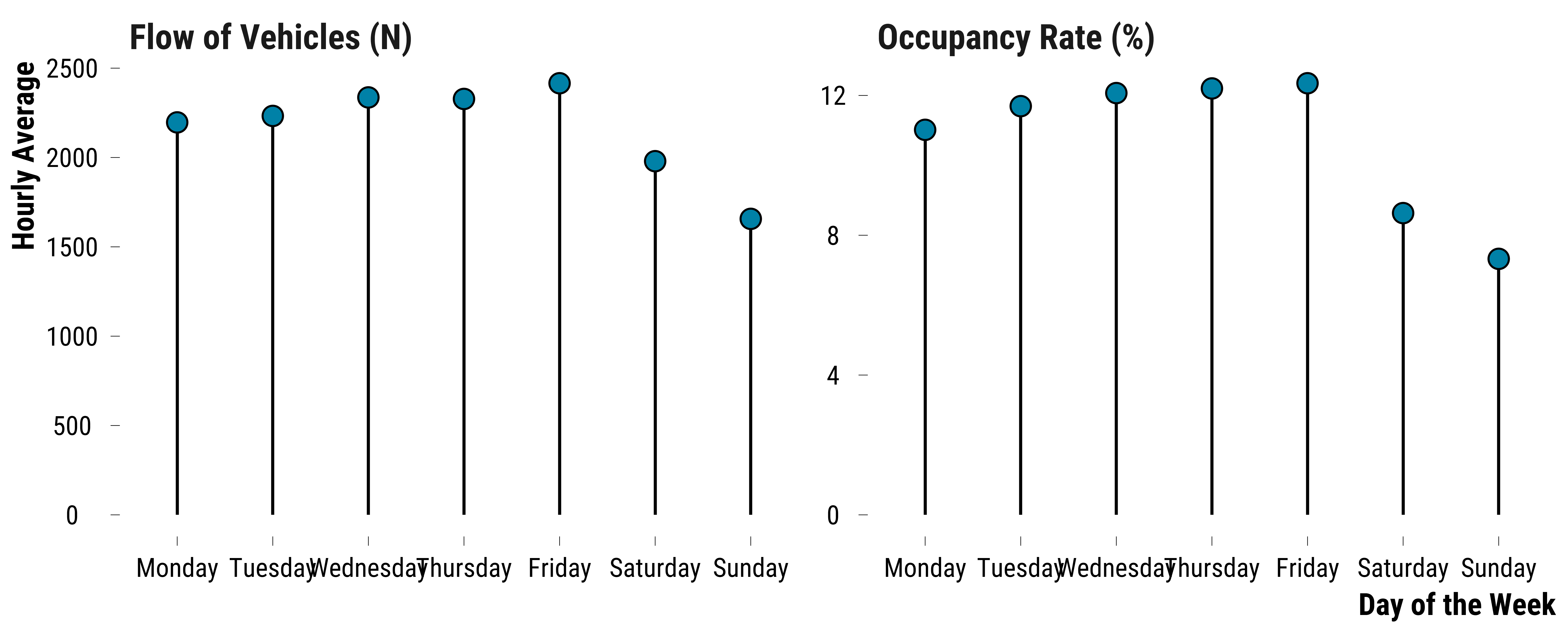
We first plot the average road traffic flow and occupancy rate by day of the week :

Please show me the code!

# make the graph
graph_road_traffic_wd <- data %>%
  select(weekday, road_traffic_flow_all, road_occupancy_rate) %>%
  pivot_longer(cols = -c(weekday), names_to = "traffic_variable", values_to = "value") %>%
  mutate(traffic_variable = ifelse(traffic_variable == "road_traffic_flow_all", "Flow of Vehicles (N)", "Occupancy Rate (%)")) %>%
  group_by(weekday, traffic_variable) %>%
  summarise(mean_value = mean(value, na.rm = TRUE)) %>%
  ggplot(., aes(x = weekday, y = mean_value)) +
  geom_segment(aes(x = weekday, xend = weekday, y = 0, yend = mean_value)) +
  geom_point(shape = 21, size = 4, colour = "black", fill = my_blue) +
  facet_wrap(~ traffic_variable, scales = "free_y") +
  xlab("Day of the Week") + ylab("Hourly Average") +
  theme_tufte()

# we print the graph
graph_road_traffic_wd

Please show me the code!

# save the graph
ggsave(
  graph_road_traffic_wd,
  filename = here::here(
    "inputs",
    "3.outputs",
    "2.daily_analysis",
    "2.analysis_pollution",
    "2.road_traffic",
    "graph_road_traffic_wd.pdf"
  ),
  width = 30,
  height = 15,
  units = "cm",
  device = cairo_pdf
)

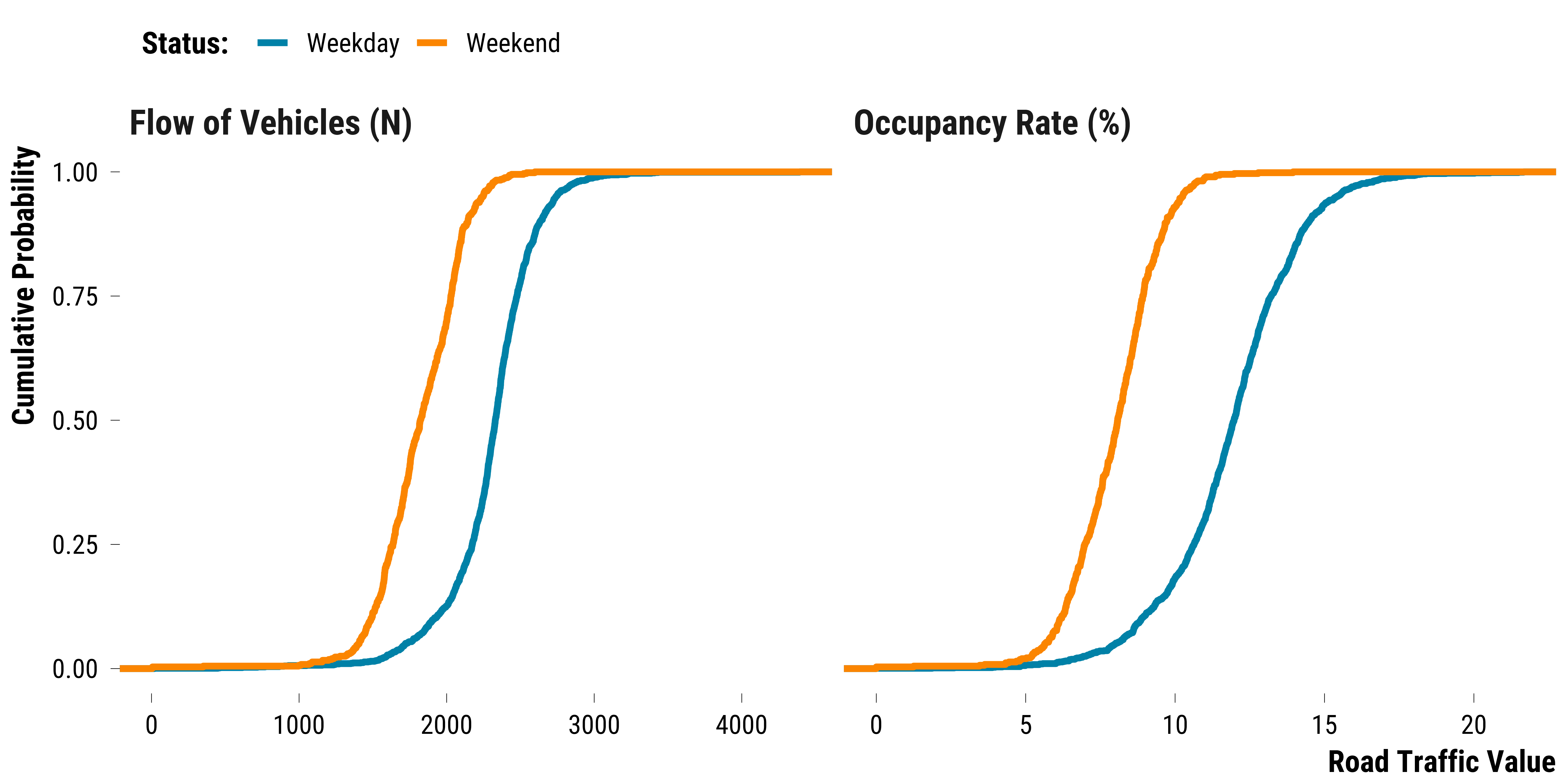
We then plot the empirical cumulative distribution of road traffic by weekdays and weekend:

Please show me the code!

graph_ecdf_road_traffic_we <- data %>%
  select(weekend, road_traffic_flow_all, road_occupancy_rate) %>%
  pivot_longer(cols = -c(weekend), names_to = "traffic_variable", values_to = "value") %>%
  mutate(traffic_variable = ifelse(traffic_variable == "road_traffic_flow_all", "Flow of Vehicles (N)", "Occupancy Rate (%)")) %>%
  mutate(weekend = ifelse(weekend == 1, "Weekend", "Weekday")) %>%
  ggplot(., aes(x = value, colour = weekend)) +
  stat_ecdf(size = 1.1) +
  scale_color_manual(values = c(my_blue, my_orange)) +
  facet_wrap(~ traffic_variable, scales = "free_x") +
  ylab("Cumulative Probability") + xlab("Road Traffic Value") +
  labs(colour = "Status:") +
  theme_tufte()

# we print the graph
graph_ecdf_road_traffic_we

Please show me the code!

# save the graph
ggsave(
  graph_ecdf_road_traffic_we,
  filename = here::here(
    "inputs",
    "3.outputs",
    "2.daily_analysis",
    "2.analysis_pollution",
    "2.road_traffic",
    "graph_ecdf_road_traffic_we.pdf"
  ),
  width = 30,
  height = 18,
  units = "cm",
  device = cairo_pdf
)

NO2 Variation by Day of the Week

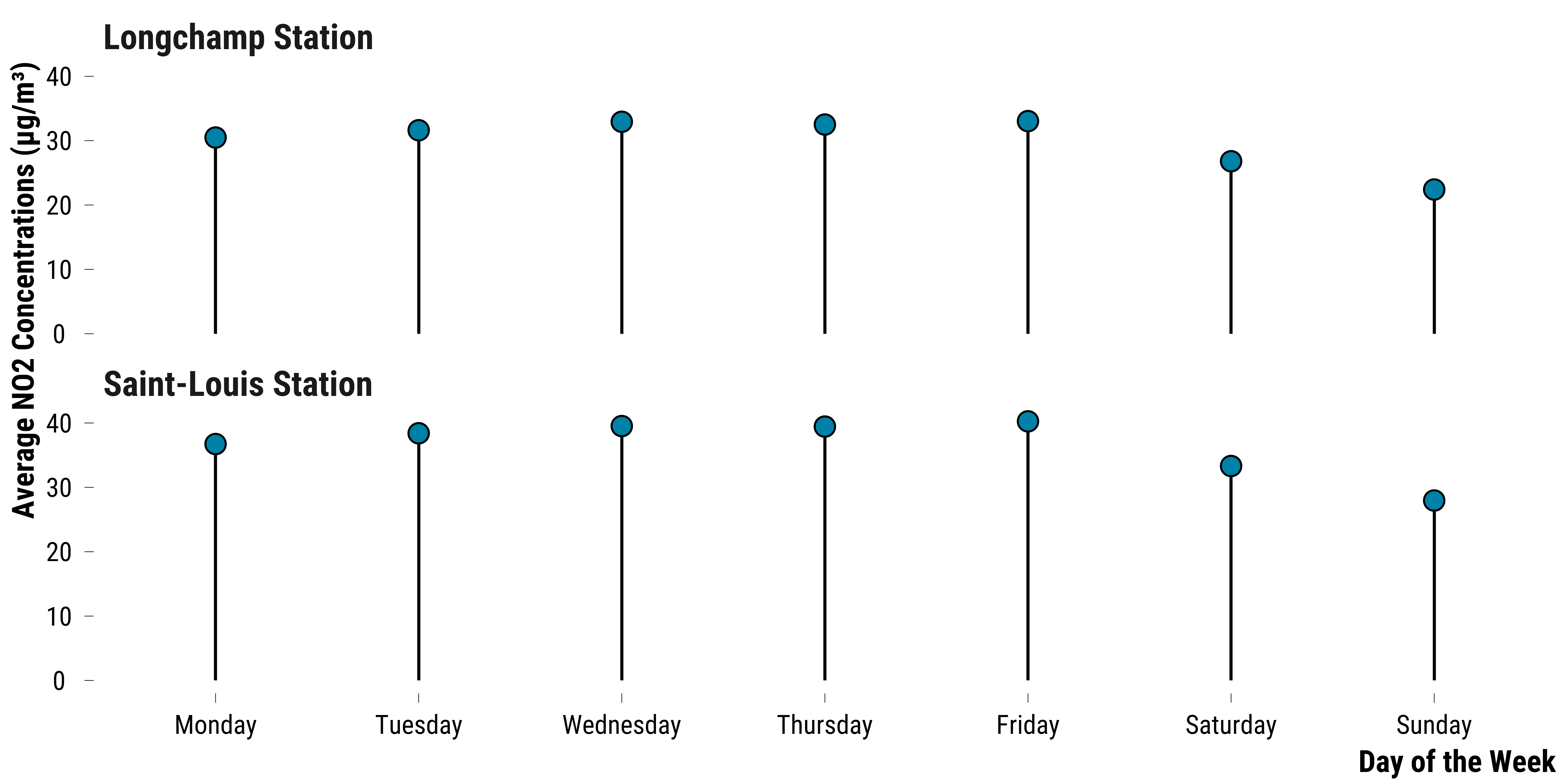
We plot the average NO2 concentration by day of the week:

Please show me the code!

# make the graph
graph_no2_wd <- data %>%
  select(weekday, mean_no2_l, mean_no2_sl) %>%
  rename("Longchamp Station" = mean_no2_l,
         "Saint-Louis Station" = mean_no2_sl) %>%
  pivot_longer(cols = -c(weekday),
               names_to = "station",
               values_to = "concentration") %>%
  group_by(weekday, station) %>%
  summarise(mean_no2 = mean(concentration, na.rm = TRUE)) %>%
  ggplot(., aes(x = weekday, y = mean_no2)) +
  geom_segment(aes(
    x = weekday,
    xend = weekday,
    y = 0,
    yend = mean_no2
  )) +
  geom_point(
    shape = 21,
    size = 4,
    colour = "black",
    fill = my_blue
  ) +
  facet_wrap( ~ station, ncol = 1) +
  xlab("Day of the Week") + ylab("Average NO2 Concentrations (µg/m³)") +
  theme_tufte()

# we print the graph
graph_no2_wd

Please show me the code!

# save the graph
ggsave(
  graph_no2_wd,
  filename = here::here(
    "inputs",
    "3.outputs",
    "2.daily_analysis",
    "2.analysis_pollution",
    "2.road_traffic",
    "graph_no2_wd.pdf"
  ),
  width = 30,
  height = 25,
  units = "cm",
  device = cairo_pdf
)

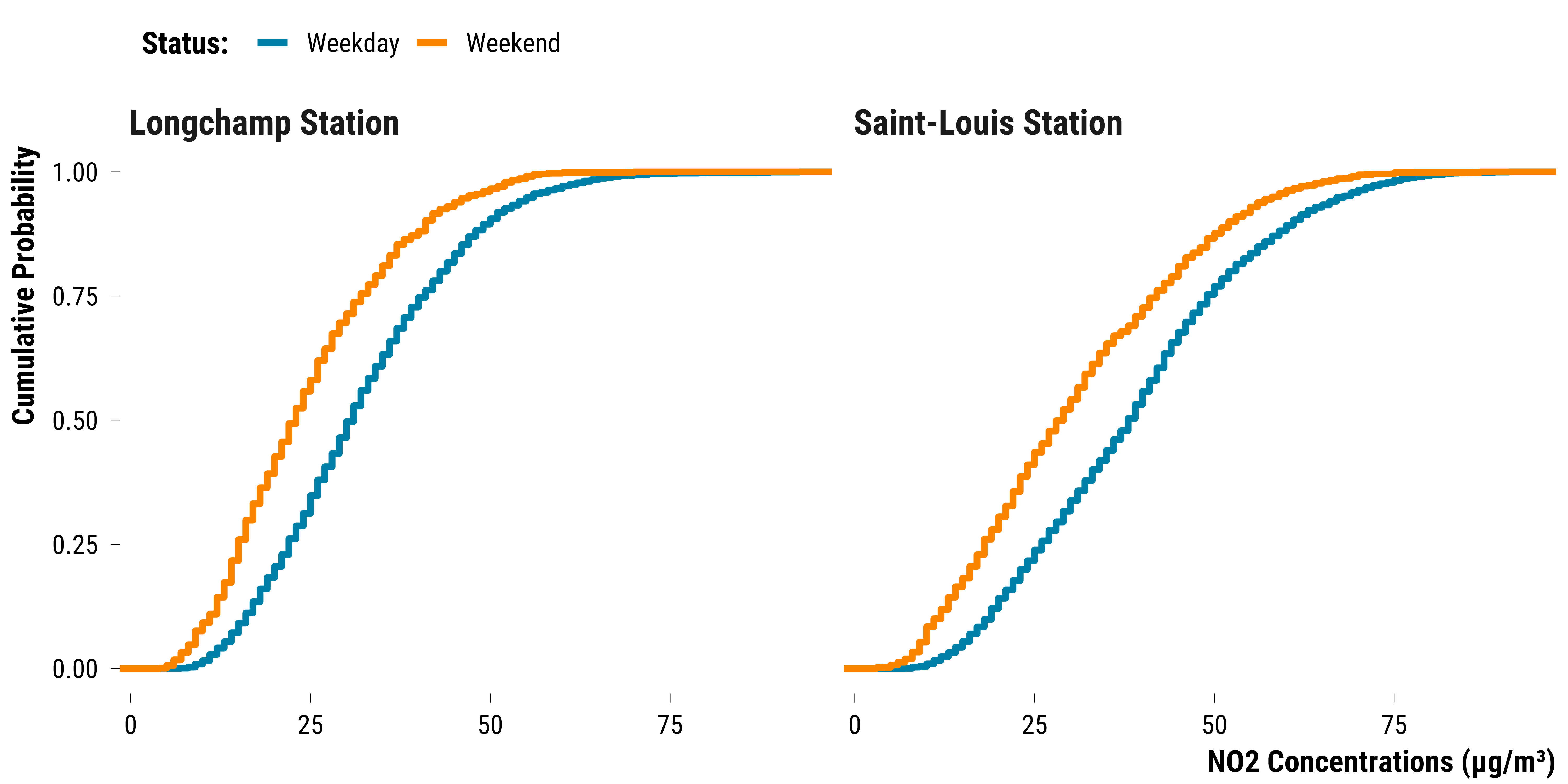
We also plot the empirical cumulative distribution of NO $_{2}$ concentration by weekdays and weekend:

Please show me the code!

# make the graph
graph_ecdf_no2_we <- data %>%
  select(weekend, mean_no2_l, mean_no2_sl) %>%
  mutate(weekend = ifelse(weekend == 1, "Weekend", "Weekday")) %>%
  rename("Longchamp Station" = mean_no2_l,
         "Saint-Louis Station" = mean_no2_sl) %>%
  pivot_longer(cols = -c(weekend),
               names_to = "station",
               values_to = "concentration") %>%
  ggplot(., aes(x = concentration, colour = weekend)) +
  stat_ecdf(size = 1.1) +
  scale_color_manual(values = c(my_blue, my_orange)) +
  facet_wrap( ~ station) +
  ylab("Cumulative Probability") + xlab("NO2 Concentrations (µg/m³)") +
  labs(colour = "Status:") +
  theme_tufte() +
  theme(
    legend.position = "top",
    legend.justification = "left",
    legend.direction = "horizontal"
  )

# we print the graph
graph_ecdf_no2_we

Please show me the code!

# save the graph
ggsave(
  graph_ecdf_no2_we,
  filename = here::here(
    "inputs",
    "3.outputs",
    "2.daily_analysis",
    "2.analysis_pollution",
    "2.road_traffic",
    "graph_ecdf_no2_we.pdf"
  ),
  width = 30,
  height = 15,
  units = "cm",
  device = cairo_pdf
)

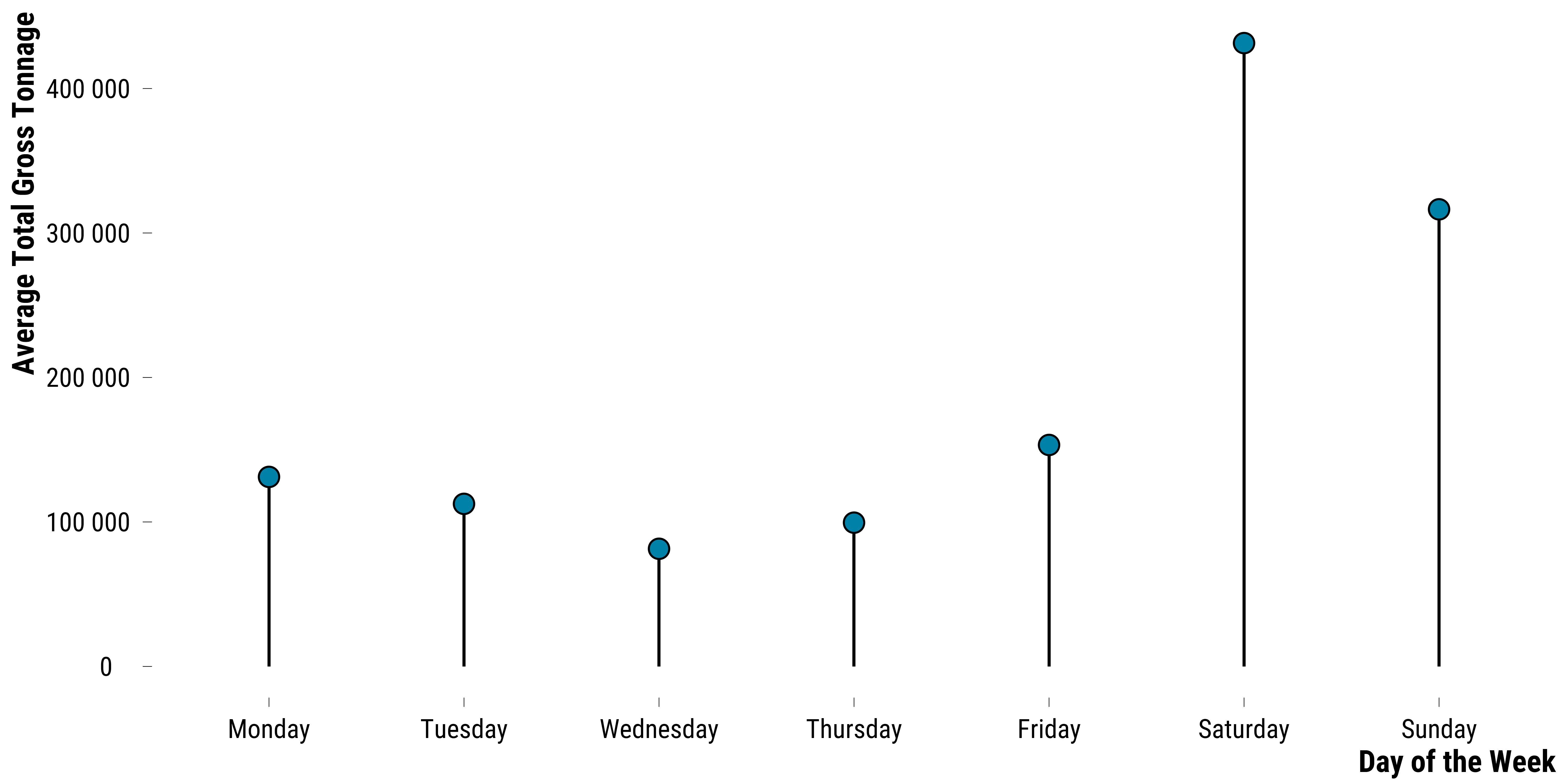
Average Total Gross Tonnage of Cruise Vessels by Day of the Week

We plot the average total gross tonnage of vessels by day of the week:

Please show me the code!

graph_gross_tonnage_cruise_wd <- data %>%
  select(weekday, total_gross_tonnage_cruise) %>%
  group_by(weekday) %>%
  summarise(total_gross_tonnage_cruise = mean(total_gross_tonnage_cruise, na.rm = TRUE)) %>%
  ggplot(., aes(x = weekday, y = total_gross_tonnage_cruise)) +
  geom_segment(aes(
    x = weekday,
    xend = weekday,
    y = 0,
    yend = total_gross_tonnage_cruise
  )) +
  geom_point(
    shape = 21,
    size = 4,
    colour = "black",
    fill = my_blue
  ) +
  scale_y_continuous(
    breaks = scales::pretty_breaks(n = 5),
    labels = function(x)
      format(x, big.mark = " ", scientific = FALSE)
  ) +
  xlab("Day of the Week") + ylab("Average Total Gross Tonnage") +
  theme_tufte()

# we print the graph
graph_gross_tonnage_cruise_wd

Please show me the code!

# save the graph
ggsave(
  graph_gross_tonnage_cruise_wd,
  filename = here::here(
    "inputs",
    "3.outputs",
    "2.daily_analysis",
    "2.analysis_pollution",
    "2.road_traffic",
    "graph_gross_tonnage_cruise_wd.pdf"
  ),
  width = 30,
  height = 15,
  units = "cm",
  device = cairo_pdf
)

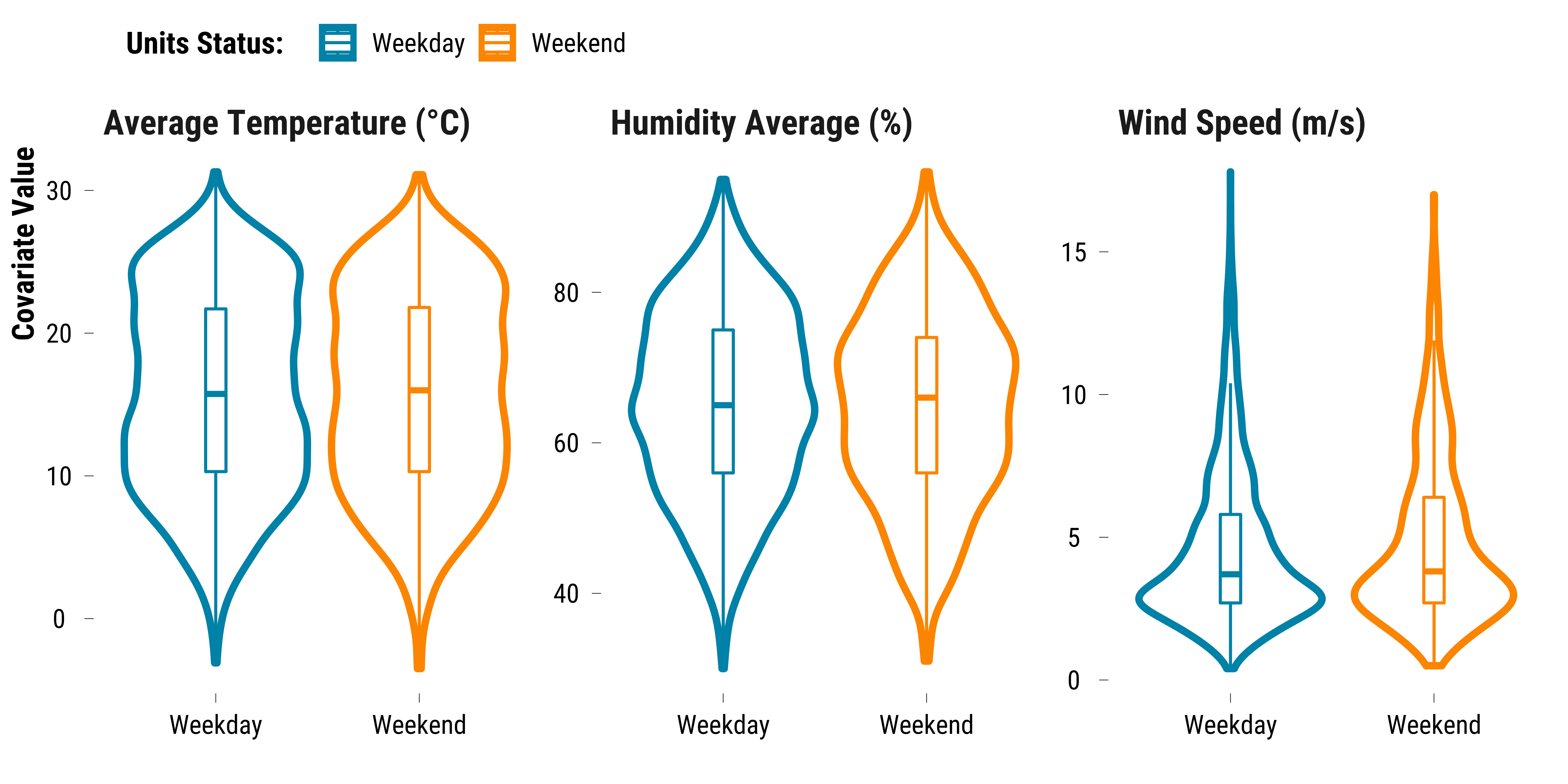
Weather Covariates Balance

We can check that the weekends and weekdays are similar for weather covariates. For continuous weather covariates, we draw boxplots for treated and control groups:

Please show me the code!

# we select control variables and store them in a long dataframe
data_weather_continuous_variables <- data %>%
  mutate(weekend = ifelse(weekend == 1, "Weekend", "Weekday")) %>%
  select(temperature_average,
         humidity_average,
         wind_speed,
         weekend) %>%
  pivot_longer(cols = -c(weekend),
               names_to = "variable",
               values_to = "values") %>%
  mutate(
    variable = case_when(
      variable == "temperature_average" ~ "Average Temperature (°C)",
      variable == "humidity_average" ~ "Humidity Average (%)",
      variable == "wind_speed" ~ "Wind Speed (m/s)"
    )
  )


graph_boxplot_continuous_weather <-
  ggplot(data_weather_continuous_variables,
         aes(x = weekend, y = values, colour = weekend)) +
  geom_violin(size = 1.2) +
  geom_boxplot(width = 0.1, outlier.shape = NA) +
  scale_color_manual(values = c(my_blue, my_orange)) +
  ylab("Covariate Value") +
  xlab("") +
  labs(colour = "Units Status:") +
  facet_wrap( ~ variable, scale = "free", ncol = 3) +
  theme_tufte() +
  theme(
    legend.position = "top",
    legend.justification = "left",
    legend.direction = "horizontal"
  )

# we print the graph
graph_boxplot_continuous_weather

Please show me the code!

# save the graph
ggsave(
  graph_boxplot_continuous_weather,
  filename = here::here(
    "inputs",
    "3.outputs",
    "2.daily_analysis",
    "2.analysis_pollution",
    "2.road_traffic",
    "graph_boxplot_continuous_weather.pdf"
  ),
  width = 40,
  height = 15,
  units = "cm",
  device = cairo_pdf
)

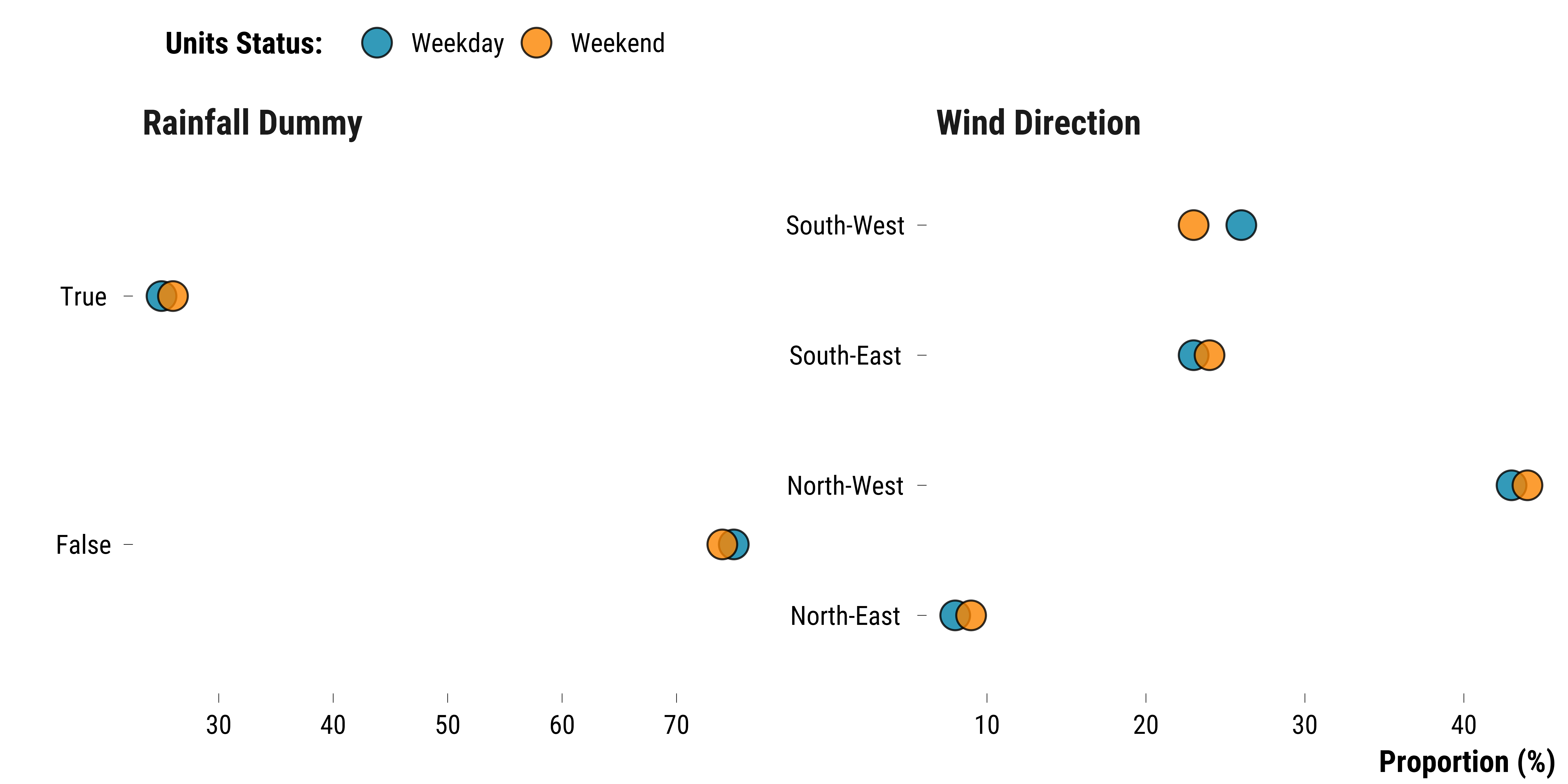
For the rainfall dummy and the wind direction categories, we plot the proportions:

Please show me the code!

# we select the rainfall variables
data_weather_categorical <- data %>%
  mutate(weekend = ifelse(weekend == 1, "Weekend", "Weekday")) %>%
  select(rainfall_height_dummy,
         wind_direction_categories,
         weekend) %>%
  drop_na() %>%
  mutate_at(vars(rainfall_height_dummy), ~ ifelse(. == 1, "True", "False")) %>%
  mutate_all(~ as.character(.)) %>%
  pivot_longer(cols = -c(weekend),
               names_to = "variable",
               values_to = "values") %>%
  # group by weekend, variable and values
  group_by(weekend, variable, values) %>%
  # compute the number of observations
  summarise(n = n()) %>%
  # compute the proportion
  mutate(freq = round(n / sum(n) * 100, 0)) %>%
  ungroup() %>%
  mutate(
    variable = case_when(
      variable == "wind_direction_categories" ~ "Wind Direction",
      variable == "rainfall_height_dummy" ~ "Rainfall Dummy"
    )
  )

# build the graph
graph_categorical_weather <-
  ggplot(data_weather_categorical, aes(x = freq, y = values, fill = weekend)) +
  geom_point(shape = 21,
             size = 6,
             alpha = 0.8) +
  scale_fill_manual(values = c(my_blue, my_orange)) +
  facet_wrap(~ variable, scales = "free") +
  xlab("Proportion (%)") +
  ylab("") +
  labs(fill = "Units Status:") +
  theme_tufte() +
  theme(
    legend.position = "top",
    legend.justification = "left",
    legend.direction = "horizontal"
  )

# we print the graph
graph_categorical_weather

Please show me the code!

# save the graph
ggsave(
  graph_categorical_weather,
  filename = here::here(
    "inputs",
    "3.outputs",
    "2.daily_analysis",
    "2.analysis_pollution",
    "2.road_traffic",
    "graph_categorical_weather.pdf"
  ),
  width = 40,
  height = 20,
  units = "cm",
  device = cairo_pdf
)

Weekend Effect on Road Traffic and NO $_{2}$ Concentrations

We calculate the average differences in road traffic and NO $_{2}$ concentrations between weekends and weekdays.

Weekend Effect on Road Traffic

We compute the average difference in the flow of vehicles and road occupancy rate between weekdays and weekends:

# compute difference in flow
diff_flow <- data %>%
  filter(!is.na(road_traffic_flow_all)) %>%
  summarise(average_difference = mean(road_traffic_flow_all[weekend == 1]) - mean(road_traffic_flow_all[weekend == 0]))

# compute difference in occupancy rate
diff_occupancy <- data %>%
  filter(!is.na(road_occupancy_rate)) %>%
  summarise(average_difference = mean(road_occupancy_rate[weekend == 1]) - mean(road_occupancy_rate[weekend == 0]))

On average, the hourly road traffic decreases by 484 vehicles on weekends. There is a drop of -3.9 poins in the occupancy rate.

Weekend Effect on NO2 concentrations

We compute the average effect of weekends on NO2 concentrations.

# compute mean difference in no2 for the two stations
diff_no2 <- data %>%
  select(weekend, mean_no2_l, mean_no2_sl) %>%
  pivot_longer(cols = -c(weekend),
               names_to = "station",
               values_to = "concentration") %>%
  group_by(station) %>%
  summarise(average_difference = round(mean(concentration[weekend == 1], na.rm = TRUE) - mean(concentration[weekend == 0], na.rm = TRUE), 1))

On average, NO $_{2}$ is lower between 7.5 and 8.2 $\mu g/m^{3}$ on weekends compared to weekdays, depending on the monitoring station.

Exploraty Data Analysis of the Effect of Road Traffic on NO2 Concentration in Marseille

Authors

Affiliations

Published

DOI

Required Packages

Data Loading and Formatting

Exploratory Data Analysis

Road Traffic Variation by Day of the Week

NO2 Variation by Day of the Week

Average Total Gross Tonnage of Cruise Vessels by Day of the Week

Weather Covariates Balance

Weekend Effect on Road Traffic and NO $_{2}$ Concentrations

Weekend Effect on Road Traffic

Weekend Effect on NO2 concentrations

Footnotes

Corrections

Exploraty Data Analysis of the Effect of Road Traffic on NO2 Concentration in Marseille

Authors

Affiliations

Published

DOI

Required Packages

Data Loading and Formatting

Exploratory Data Analysis

Road Traffic Variation by Day of the Week

NO2 Variation by Day of the Week

Average Total Gross Tonnage of Cruise Vessels by Day of the Week

Weather Covariates Balance

Weekend Effect on Road Traffic and NO2_{2} Concentrations

Weekend Effect on Road Traffic

Weekend Effect on NO2 concentrations

Footnotes

Corrections

Weekend Effect on Road Traffic and NO $_{2}$ Concentrations