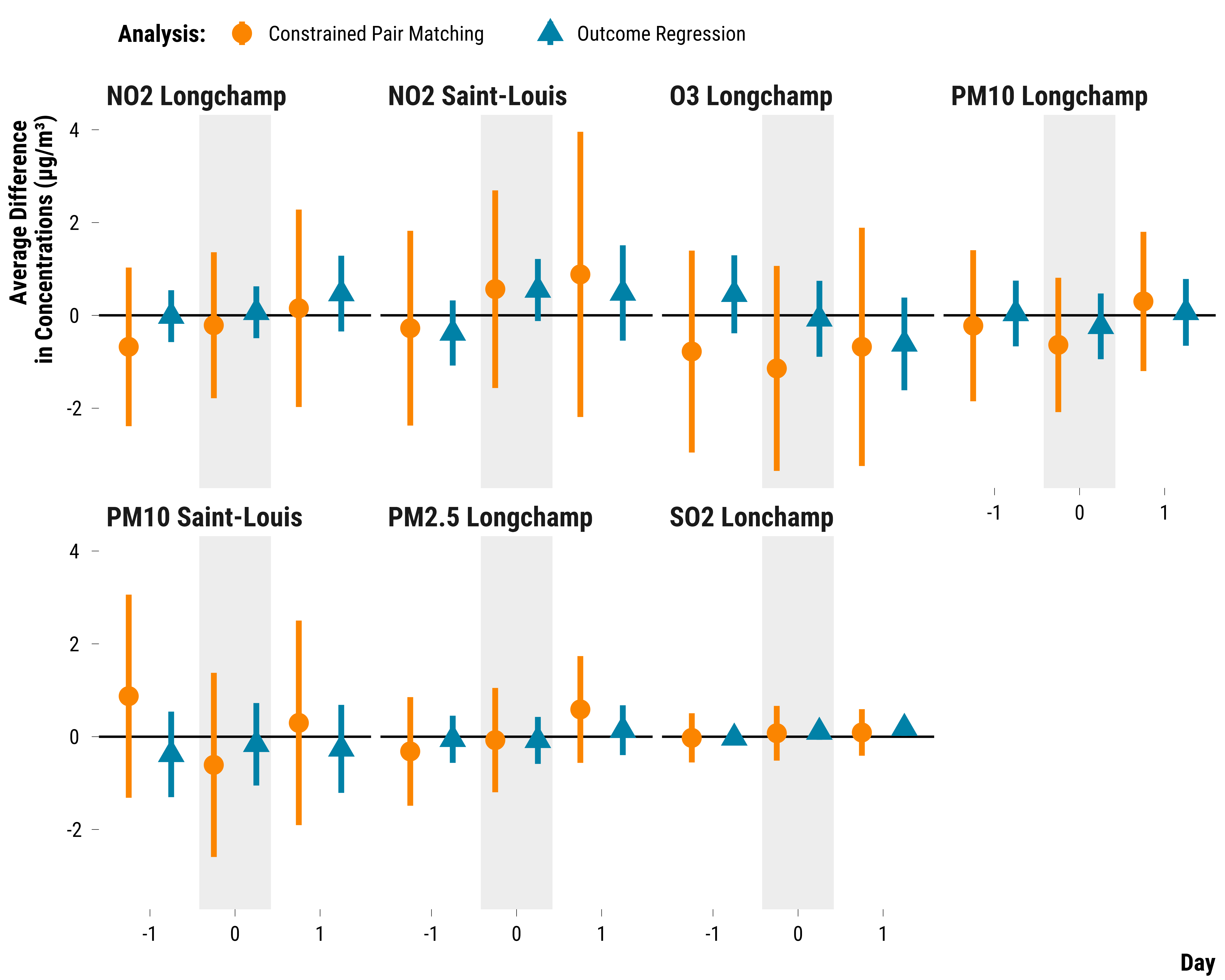
In this document, we compare the results found with our matching analysis with those found with an outcome regression approach.
Should you have any questions, need help to reproduce the analysis or find coding errors, please do not hesitate to contact us at leo.zabrocki@gmail.com and marion.leroutier@hhs.se.
Required Packages and Data
We load the following packages:
# load required packages
library(knitr) # for creating the R Markdown document
library(here) # for files paths organization
library(tidyverse) # for data manipulation and visualization
library(broom) # for cleaning regression outputs
library(randChecks) # for randomization check
library(lmtest) # for modifying regression standard errors
library(sandwich) # for robust and cluster robust standard errors
library(kableExtra) # for table formatting
library(Cairo) # for printing custom police of graphs
We load our custom ggplot2 theme for graphs:
And we load the matching data:
# load matching data
data_matching <-
  readRDS(
    here::here(
      "inputs",
      "1.data",
      "2.daily_data",
      "2.data_for_analysis",
      "1.cruise_experiment",
      "matching_data.rds"
    )
  ) %>%
  mutate(year = as.factor(year)) %>%
  select(
    is_treated,
    year,
    month,
    weekday,
    holidays_dummy,
    bank_day_dummy,
    total_gross_tonnage_ferry:total_gross_tonnage_other_boat,
    temperature_average:wind_speed,
    wind_direction_east_west,
    holidays_dummy_lag_1,
    bank_day_dummy_lag_1,
    total_gross_tonnage_cruise_lag_1:total_gross_tonnage_other_boat_lag_1,
    temperature_average_lag_1:wind_speed_lag_1,
    wind_direction_east_west_lag_1,
    contains("no2"),
    contains("o3"),
    contains("pm10"),
    contains("pm25"),
    contains("so2")
  )
Balance check
We first evaluate as the overall balance of our treatment before matching by implementing the randomization inference approach proposed by Zach Branson (2021):
# we select covariates
data_covs <- data_matching %>%
  select(
    is_treated,
    year,
    month,
    weekday,
    holidays_dummy,
    bank_day_dummy,
    total_gross_tonnage_ferry:total_gross_tonnage_other_boat,
    temperature_average:wind_speed,
    wind_direction_east_west,
    holidays_dummy_lag_1,
    bank_day_dummy_lag_1,
    total_gross_tonnage_cruise_lag_1:total_gross_tonnage_other_boat_lag_1,
    temperature_average_lag_1:wind_speed_lag_1,
    wind_direction_east_west_lag_1,
    mean_no2_l_lag_1:mean_o3_l_lag_1
  ) %>%
  drop_na()

data_covs <- data_covs %>%
  group_by(year, month) %>%
  mutate(year_month_block = cur_group_id())

# recode some variables
data_covs <- data_covs %>%
  mutate(is_treated = ifelse(is_treated == TRUE, 1, 0)) %>%
  mutate_at(
    vars(wind_direction_east_west , wind_direction_east_west_lag_1),
    ~ ifelse(. == "West", 1, 0)
  ) %>%
  fastDummies::dummy_cols(., select_columns = c("year", "month", "weekday")) %>%
  select(-c("year", "month", "weekday"))

# format data for asIfRandPlot() function
is_treated <- data_covs$is_treated
year_month_block <- data_covs$year_month_block

data_covs <- data_covs %>%
  select(-is_treated, -year_month_block) %>%
  select(-year_2018,-month_December, -weekday_Sunday)

# run balance check
asIfRandPlot(
  X.matched = data_covs,
  indicator.matched = is_treated,
  assignment = c("complete", "blocked"),
  subclass = year_month_block,
  perms = 1000
)

Regression Analysis
We run an outcome regression analysis where we regress the concentration of air pollutants on the treatment indiciator, measures of other vessels traffic, weather parameters and calendar indicators:
Please show me the code!
# define outcome regression function
function_reg_analysis <- function(data) {
  # we fit the regression model
  model <-
    lm(
      concentration ~ is_treated + total_gross_tonnage_ferry + total_gross_tonnage_other_boat +
        total_gross_tonnage_ferry_lag_1 + total_gross_tonnage_other_boat_lag_1 +
        temperature_average + temperature_average_lag_1 +
        humidity_average + humidity_average_lag_1 +
        rainfall_height_dummy + rainfall_height_dummy_lag_1 +
        wind_direction_east_west + wind_direction_east_west_lag_1 +
        wind_speed + wind_speed_lag_1 +
        weekday + holidays_dummy + bank_day_dummy + month * year,
      data = data
    )

  # retrieve the estimate and 95% ci
  results_reg <- tidy(coeftest(model, vcov = vcovHC),
                      conf.int = TRUE) %>%
    filter(term == "is_treatedTRUE") %>%
    select(term, estimate, conf.low, conf.high)

  # return output
  return(results_reg)
}

# reshape in long according to pollutants
data_reg_analysis <- data_matching %>%
  pivot_longer(cols = c(contains("no2"), contains("o3"), contains("pm10"), contains("pm25"), contains("so2")), names_to = "variable", values_to = "concentration") %>%
  mutate(pollutant = NA %>%
           ifelse(str_detect(variable, "no2_l"), "NO2 Longchamp",.) %>%
           ifelse(str_detect(variable, "no2_sl"), "NO2 Saint-Louis",.) %>%
           ifelse(str_detect(variable, "o3"), "O3 Longchamp",.) %>%
           ifelse(str_detect(variable, "pm10_l"), "PM10 Longchamp",.) %>%
           ifelse(str_detect(variable, "pm10_sl"), "PM10 Saint-Louis",.) %>%
           ifelse(str_detect(variable, "pm25"), "PM2.5 Longchamp",.) %>%
           ifelse(str_detect(variable, "so2"), "SO2 Lonchamp",.)) %>%
  mutate(time = 0 %>%
           ifelse(str_detect(variable, "lag_1"), -1, .) %>%
           ifelse(str_detect(variable, "lead_1"), 1, .)) %>%
  select(-variable)

# we nest the data by pollutant and time
data_reg_analysis <- data_reg_analysis %>%
  group_by(pollutant, time) %>%
  nest()

# run outcome regression analysis
data_reg_analysis <- data_reg_analysis %>%
  mutate(result = map(data, ~ function_reg_analysis(.))) %>%
  select(-data) %>%
  unnest(cols = c(result)) %>%
  select(-term) %>%
  rename("mean_difference" = "estimate", "ci_lower_95" = "conf.low", "ci_upper_95" = "conf.high") %>%
  mutate(analysis = "Outcome Regression")

# load matching results
data_neyman <- readRDS(
  here(
    "inputs",
    "1.data",
    "2.daily_data",
    "2.data_for_analysis",
    "1.cruise_experiment",
    "data_neyman.rds"
  )
)

data_neyman <- data_neyman %>%
  mutate(analysis = "Constrained Pair Matching")

# merge them with outcome regression results
data_neyman_reg <- bind_rows(data_neyman, data_reg_analysis)

# create an indicator to alternate shading of confidence intervals
data_neyman_reg <- data_neyman_reg %>%
  arrange(pollutant, time) %>%
  mutate(stripe = ifelse((time %% 2) == 0, "Grey", "White")) %>%
  ungroup()

# make the graph
graph_reg_analysis <-
  ggplot(
    data_neyman_reg,
    aes(
      x = as.factor(time),
      y = mean_difference,
      ymin = ci_lower_95,
      ymax = ci_upper_95,
      colour = analysis,
      shape = analysis
    )
  ) +
  geom_rect(
    aes(fill = stripe),
    xmin = as.numeric(as.factor(data_neyman_reg$time)) - 0.42,
    xmax = as.numeric(as.factor(data_neyman_reg$time)) + 0.42,
    ymin = -Inf,
    ymax = Inf,
    color = NA,
    alpha = 0.4
  ) +
  geom_hline(yintercept = 0, color = "black") +
  geom_pointrange(position = position_dodge(width = 1), size = 1.2) +
  scale_shape_manual(name = "Analysis:", values = c(16, 17)) +
  scale_color_manual(name = "Analysis:", values = c(my_orange, my_blue)) +
  facet_wrap( ~ pollutant, ncol = 4) +
  scale_fill_manual(values = c('grey90', "white")) +
  guides(fill = FALSE) +
  ylab("Average Difference \nin Concentrations (µg/m³)") + xlab("Day") +
  theme_tufte()

# display the graph
graph_reg_analysis
Please show me the code!
# save the graph
ggsave(
  graph_reg_analysis + labs(title = NULL),
  filename = here::here(
    "inputs",
    "3.outputs",
    "2.daily_analysis",
    "2.analysis_pollution",
    "1.cruise_experiment",
    "3.outcome_regression",
    "graph_reg_analysis.pdf"
  ),
  width = 30,
  height = 15,
  units = "cm",
  device = cairo_pdf
)