Matching Procedure

Comparing days with cruise traffic to days without. Adjusting for calendar and weather indicators.

In this document, we provide all steps required to reproduce our matching procedure at the daily level. We compare days where:

• treated units are days with cruise traffic in t.
• control units are day without cruise traffic in t.

We adjust for calendar calendar indicator and weather confounding factors.

Should you have any questions, need help to reproduce the analysis or find coding errors, please do not hesitate to contact us at leo.zabrocki@gmail.com and marion.leroutier@hhs.se.

Required Packages

We load the following packages:

# load required packages
library(knitr) # for creating the R Markdown document
library(here) # for files paths organization
library(tidyverse) # for data manipulation and visualization
library(Rcpp) # for running the matching algorithm
library(optmatch) # for matching pairs
library(igraph) # for pair matching via bipartite maximal weighted matching
library(kableExtra) # for table formatting

We also have to load the script_time_series_matching_function.R which provides the functions used for matching time series:

# load matching functions
source(here::here(
  "inputs",
  "2.functions",
  "script_time_series_matching_function.R"
))

We finally load our custom ggplot2 theme for graphs:

# load ggplot custom theme
source(here::here(
  "inputs",
  "2.functions",
  "script_theme_tufte.R"
))
# define nice colors
my_blue <- "#0081a7"
my_orange <- "#fb8500"

Preparing the Data for Matching

Selecting and Creating Relevant Variables

First, we load the data:

# load data
data <-
  readRDS(
    here::here(
      "inputs",
      "1.data",
      "2.daily_data",
      "2.data_for_analysis",
      "0.main_data",
      "data_for_analysis_daily.RDS"
    )
  )

Then, we select relevant variables for matching and create new variables which we store in the processed_data:

# select relevant variables
relevant_variables <- c(
  "date",
  "mean_no2_l",
  "mean_no2_sl",
  "mean_pm10_l",
  "mean_pm10_sl",
  "mean_pm25_l",
  "mean_so2_l",
  "mean_o3_l",
  "total_gross_tonnage",
  "total_gross_tonnage_cruise",
  "total_gross_tonnage_ferry",
  "total_gross_tonnage_other_boat",
  "temperature_average",
  "rainfall_height_dummy",
  "humidity_average",
  "wind_speed",
  "wind_direction_categories",
  "wind_direction_east_west",
  "road_traffic_flow_all",
  "road_occupancy_rate",
  "weekday",
  "weekend",
  "holidays_dummy",
  "bank_day_dummy",
  "month",
  "season",
  "year"
)

# create processed_data with the relevant variables
if (exists("relevant_variables") && !is.null(relevant_variables)) {
  # extract relevant variables (if specified)
  processed_data = data[relevant_variables]
} else {
  processed_data = data
}

# create julian date and day of the year to define time windows
processed_data <- processed_data %>%
  mutate(julian_date = julian(date),
         day_of_year = lubridate::yday(date))

#
# re-order columns
#

processed_data <- processed_data %>%
  select(
    # date variable
    "date",
    # pollutants
    "mean_no2_l",
    "mean_no2_sl",
    "mean_pm10_l",
    "mean_pm10_sl",
    "mean_pm25_l",
    "mean_so2_l",
    "mean_o3_l",
    # maritime traffic variables
    "total_gross_tonnage",
    "total_gross_tonnage_cruise",
    "total_gross_tonnage_ferry",
    "total_gross_tonnage_other_boat",
    # weather parameters
    "temperature_average",
    "rainfall_height_dummy",
    "humidity_average",
    "wind_speed",
    "wind_direction_categories",
    "wind_direction_east_west",
    # road traffic variables
    "road_traffic_flow_all",
    "road_occupancy_rate",
    # calendar indicators
    "julian_date",
    "day_of_year",
    "weekday",
    "weekend",
    "holidays_dummy",
    "bank_day_dummy",
    "month",
    "season",
    "year"
  )

For each covariate, we create the first daily lags and leads:

# we first define processed_data_leads and processed_data_lags
# to store leads and lags

processed_data_leads <- processed_data
processed_data_lags <- processed_data

#
# create leads
#

# create a list to store dataframe of leads
leads_list <- vector(mode = "list", length = 1)
names(leads_list) <- c(1)

# create the leads
for (i in 1) {
  leads_list[[i]] <- processed_data_leads %>%
    mutate_at(vars(-date), ~  lead(., n = i, order_by = date)) %>%
    rename_at(vars(-date), function(x)
      paste0(x, "_lead_", i))
}

# merge the dataframes of leads
data_leads <- leads_list %>%
  reduce(left_join, by = "date")

# merge the leads with the processed_data_leads
processed_data_leads <-
  left_join(processed_data_leads, data_leads, by = "date") %>%
  select(-c(mean_no2_l:year))

#
# create lags
#

# create a list to store dataframe of lags
lags_list <- vector(mode = "list", length = 1)
names(lags_list) <- c(1)

# create the lags
for (i in 1) {
  lags_list[[i]] <- processed_data_lags %>%
    mutate_at(vars(-date), ~  lag(., n = i, order_by = date)) %>%
    rename_at(vars(-date), function(x)
      paste0(x, "_lag_", i))
}

# merge the dataframes of lags
data_lags <- lags_list %>%
  reduce(left_join, by = "date")

# merge the lags with the initial processed_data_lags
processed_data_lags <-
  left_join(processed_data_lags, data_lags, by = "date")

#
# merge processed_data_leads with processed_data_lags
#

processed_data <-
  left_join(processed_data_lags, processed_data_leads, by = "date")

We can now define the hypothetical experiment that we would like to investigate.

Creating Potential Experiments

We defined our potential experiments such that:

• treated units are days with cruise traffic in t.
• control units are day without cruise traffic in t.

Below are the required steps to select the corresponding treated and control units whose observations are stored in the matching_data:

# construct treatment assigment variable
processed_data <- processed_data %>%
  mutate(is_treated = NA) %>%
  mutate(is_treated = ifelse(total_gross_tonnage_cruise > 0, TRUE, is_treated)) %>%
  mutate(is_treated = ifelse(total_gross_tonnage_cruise == 0 , FALSE, is_treated))

# remove the days for which assignment is undefined
matching_data = processed_data[!is.na(processed_data$is_treated), ]

# susbet treated and control units
treated_units = subset(matching_data, is_treated)
control_units = subset(matching_data, !is_treated)
N_treated = nrow(treated_units)
N_control = nrow(control_units)

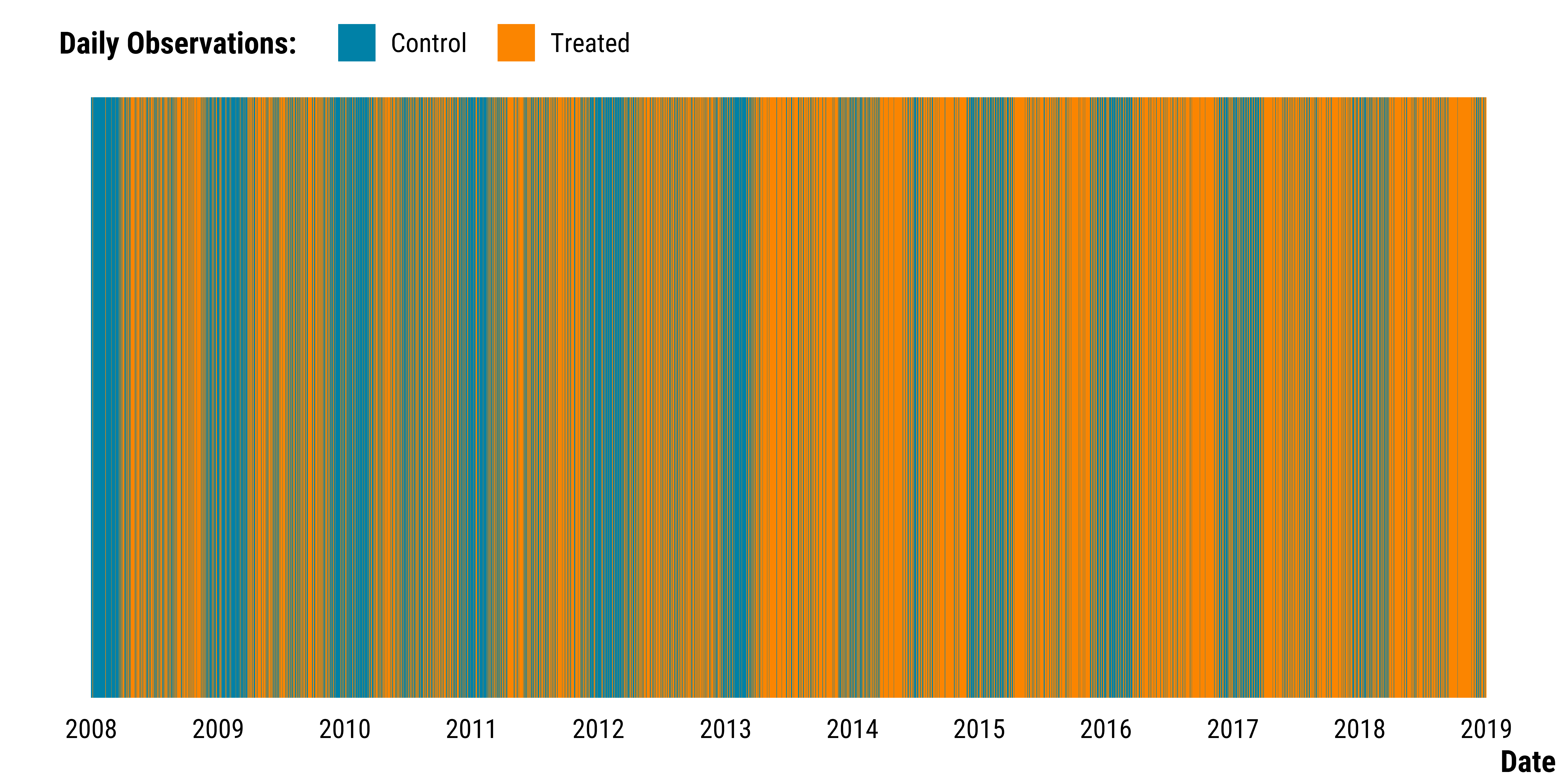
There are 2485 treated units and 1532 control units. We display the distribution of treated and control units through time:

Please show me the code!

# make stripes graph
graph_stripes_daily_experiment <- matching_data %>%
  mutate(is_treated = ifelse(is_treated == "TRUE", "Treated", "Control")) %>%
  ggplot(., aes(x = date, y = 1, fill = is_treated)) +
  geom_tile() +
  scale_x_date(breaks = scales::pretty_breaks(n = 10)) +
  scale_y_continuous(expand = c(0, 0)) +
  scale_fill_manual(name = "Daily Observations:", values = c(my_blue, my_orange)) +
  xlab("Date") +
  theme_tufte() +
  theme(
    panel.grid.major.y = element_blank(),
    axis.ticks.x = element_blank(),
    axis.ticks.y = element_blank(),
    axis.title.y = element_blank(),
    axis.text.y = element_blank()
  )

# display the graph
graph_stripes_daily_experiment

Please show me the code!

# save the graph
ggsave(
  graph_stripes_daily_experiment,
  filename = here::here(
    "inputs",
    "3.outputs",
    "2.daily_analysis",
    "2.analysis_pollution",
    "1.cruise_experiment",
    "1.checking_matching_procedure",
    "graph_stripes_daily_experiment.pdf"
  ),
  width = 30,
  height = 10,
  units = "cm",
  device = cairo_pdf
)

We save the matching_data :

# save the matching data
saveRDS(
  matching_data,
  here::here(
    "inputs",
    "1.data",
    "2.daily_data",
    "2.data_for_analysis",
    "1.cruise_experiment",
    "matching_data.RDS"
  )
)

Matching Procedure

Defining Thresholds for Matching Covariates

Below is the code to define the relevant thresholds:

# we create the scaling list as it is needed for running the algorithm
# but we do not use it

scaling =  rep(list(1), ncol(matching_data))
names(scaling) = colnames(matching_data)

# instead, we manually defined the threshold for each covariate
thresholds = rep(list(Inf), ncol(matching_data))
names(thresholds) = colnames(matching_data)

# threshold for weekday
thresholds$weekday = 0

# threshold for holidays
thresholds$holidays_dummy = 0
thresholds$holidays_dummy_lag_1 = 0

# threshold for bank days
thresholds$bank_day_dummy = 0
thresholds$bank_day_dummy_lag_1 = 0

# threshold for distance in julian days
thresholds$julian_date = 1095

# threshold for month
thresholds$month = 0

# thresholds for average temperature
thresholds$temperature_average = 4
thresholds$temperature_average_lag_1 = 4

# threshold for wind speed
thresholds$wind_speed = 2
thresholds$wind_speed_lag_1 = 2

# threshold for east-west wind direction dummy
thresholds$wind_direction_east_west = 0
thresholds$wind_direction_east_west_lag_1 = 0

# threshold for rainfall height dummy
thresholds$rainfall_height_dummy = 0
thresholds$rainfall_height_dummy_lag_1 = 0

Running the Matching Procedure

We compute discrepancy matrix and run the matching algorithm:

# first we compute the discrepancy matrix
discrepancies = discrepancyMatrix(treated_units, control_units, thresholds, scaling)

# convert matching data to data.frame
matching_data <- as.data.frame(matching_data)

rownames(discrepancies) = format(matching_data$date[which(matching_data$is_treated)], "%Y-%m-%d")
colnames(discrepancies) = format(matching_data$date[which(!matching_data$is_treated)], "%Y-%m-%d")
rownames(matching_data) = matching_data$date

# run the fullmatch algorithm
matched_groups = fullmatch(
  discrepancies,
  data = matching_data,
  remove.unmatchables = TRUE,
  max.controls = 1
)

# get list of matched  treated-control groups
groups_labels = unique(matched_groups[!is.na(matched_groups)])
groups_list = list()
for (i in 1:length(groups_labels)) {
  IDs = names(matched_groups)[(matched_groups == groups_labels[i])]
  groups_list[[i]] = as.Date(IDs[!is.na(IDs)])
}

For some cases, several controls units were matched to a treatment unit. We use the igraph package to force pair matching via bipartite maximal weighted matching. Below is the required code:

# we build a bipartite graph with one layer of treated nodes, and another layer of control nodes.
# the nodes are labeled by integers from 1 to (N_treated + N_control)
# by convention, the first N_treated nodes correspond to the treated units, and the remaining N_control
# nodes correspond to the control units.

# build pseudo-adjacency matrix: edge if and only if match is admissible
# NB: this matrix is rectangular so it is not per say the adjacendy matrix of the graph
# (for this bipartite graph, the adjacency matrix had four blocks: the upper-left block of size
# N_treated by N_treated filled with 0's, bottom-right block of size N_control by N_control filled with 0's,
# top-right block of size N_treated by N_control corresponding to adj defined below, and bottom-left block
# of size N_control by N_treated corresponding to the transpose of adj)
adj = (discrepancies<Inf)

# extract endpoints of edges
edges_mat = which(adj,arr.ind = TRUE)

# build weights, listed in the same order as the edges (we use a decreasing function x --> 1/(1+x) to
# have weights inversely proportional to the discrepancies, since maximum.bipartite.matching
# maximizes the total weight and we want to minimize the discrepancy)
weights = 1/(1+sapply(1:nrow(edges_mat),function(i)discrepancies[edges_mat[i,1],edges_mat[i,2]]))

# format list of edges (encoded as a vector resulting from concatenating the end points of each edge)
# i.e c(edge1_endpoint1, edge1_endpoint2, edge2_endpoint1, edge2_endpoint1, edge3_endpoint1, etc...)
edges_mat[,"col"] = edges_mat[,"col"] + N_treated
edges_vector = c(t(edges_mat))

# NB: by convention, the first N_treated nodes correspond to the treated units, and the remaining N_control
# nodes correspond to the control units (hence the "+ N_treated" to shift the labels of the control nodes)

# build the graph from the list of edges
BG = make_bipartite_graph(c(rep(TRUE,N_treated),rep(FALSE,N_control)), edges = edges_vector)

# find the maximal weighted matching
MBM = maximum.bipartite.matching(BG,weights = weights)

# list the dates of the matched pairs
pairs_list = list()
N_matched = 0
for (i in 1:N_treated){
  if (!is.na(MBM$matching[i])){
    N_matched = N_matched + 1
    pairs_list[[N_matched]] = c(treated_units$date[i],control_units$date[MBM$matching[i]-N_treated])
  }
}

# transform the list of matched pairs to a dataframe
matched_pairs <- enframe(pairs_list) %>%
  unnest(cols = "value") %>%
  rename(pair_number = name,
         date = value)

The hypothetical experiment we set up had 2485 treated units and 1532 control units. The matching procedure results in 189 matched treated units. We remove pairs separated by less than 7 days to avoid spillover effects within a pair:

# define distance for days
threshold_day = 6

# define distance for months
threshold_month_low = 3
threshold_month_high = 9

# find pairs that should be removed
pairs_to_remove <- matched_pairs %>%
  mutate(month = lubridate::month(date)) %>%
  #  compute pair differences in days and months
  group_by(pair_number) %>%
  summarise(
    difference_days = abs(date - dplyr::lag(date)),
    difference_month = abs(month - dplyr::lag(month))
  ) %>%
  drop_na() %>%
  # select pair according to the criteria
  mutate(day_criteria = ifelse(difference_days < threshold_day, 1, 0)) %>%
  mutate(
    month_criteria = ifelse(
      difference_month > threshold_month_low &
        difference_month < threshold_month_high,
      1,
      0
    )
  ) %>%
  filter(day_criteria == 0 & month_criteria == 0) %>%
  pull(pair_number)


# remove these pairs
matched_pairs <- matched_pairs %>%
  filter(pair_number  %in% pairs_to_remove)

We then merge the matched_pairs with the matching_matching_data to retrieve covariate values for the matched pairs:

# select the matched data for the analysis
final_data <- left_join(matched_pairs, matching_data, by = "date")

Our final number of matched treated days is therefore 189. The distribution of difference in days within a pair is summarized below:

Please show me the code!

final_data %>%
  group_by(pair_number) %>%
  summarise(difference_days = abs(date[1]-date[2])) %>%
  summarise(
    "Mean" = round(mean(difference_days, na.rm = TRUE), 1),
    "Standard Deviation" = round(sd(difference_days, na.rm = TRUE), 1),
    "Minimum" = round(min(difference_days, na.rm = TRUE), 1),
    "Maximum" = round(max(difference_days, na.rm = TRUE), 1)
  ) %>%
  # print the table
  kable(., align = c("l", rep("c", 4))) %>%
  kable_styling(position = "center")

Mean	Standard Deviation	Minimum	Maximum
470.9 days	352.6	7 days	1092 days

In the match dataset, there could however be spillover between pairs. For example, the first lead of a treated pollutant concentration could be used as a control in another pair. We first compute below the minimum of the distance of each treated unit with all other control units and then retrieve the proportion of treated units for which the minimum distance with a control unit in another pair is equal to 1 day.

Please show me the code!

# retrieve dates of treated units
treated_pairs <- final_data %>%
  select(pair_number, is_treated, date) %>%
  filter(is_treated == TRUE)

# retrieve dates of controls
control_pairs <- final_data %>%
  select(pair_number, is_treated, date) %>%
  filter(is_treated == FALSE)

# compute proportion for which the distance is 1
distance_1_day <- treated_pairs %>% 
  group_by(pair_number, date) %>%
  expand(other_date = control_pairs$date) %>%
  filter(date!=other_date) %>%
  mutate(difference = abs(date-other_date)) %>%
  group_by(pair_number) %>%
  summarise(min_difference = min(difference)) %>%
  arrange(min_difference) %>%
  summarise(sum(min_difference<=1)/n()*100)

21.7% of pairs could suffer from a between spillover effect.

We finally save the data:

# save the matched data
saveRDS(
  final_data,
  here::here(
    "inputs",
    "1.data",
    "2.daily_data",
    "2.data_for_analysis",
    "1.cruise_experiment",
    "matched_data.RDS"
  )
)