Toy Example for Understanding Randomization Inference

How to Compute Fisherian Intervals?

In this document, we explain with a toy example how to:

• Test the sharp null hypothesis of no effect for all units.
• Carry out a test inversion procedure to compute a 95% Fisherian interval for constant treatment effects consistent with the data.
• Compare the results with Neyman’s approach targeting the average causal effect.
• Adapt the randomization inference for testing weak null hypotheses (i.e., average causal effects).

Should you have any questions, need help to reproduce the analysis or find coding errors, please do not hesitate to contact us at leo.zabrocki@gmail.com and marion.leroutier@hhs.se.

Required Packages

We load the following packages:

# load required packages
library(knitr) # for creating the R Markdown document
library(here) # for files paths organization
library(tidyverse) # for data manipulation and visualization
library(kableExtra) # for building nice tables
library(Cairo) # for printing custom police of graphs

We finally load our custom ggplot2 theme for graphs:

# load ggplot custom theme
source(here::here(
  "inputs",
  "2.functions",
  "script_theme_tufte.R"
))
# define nice colors
my_blue <- "#0081a7"
my_orange <- "#fb8500"

Toy Example

In this toy example, we aim to estimate the effect of cruise vessels docking at Marseille’s port on NO\(_{2}\) concentration:

• For simplicity, imagine that our matching procedure resulted in 10 pairs of hours with similar weather and calendar characteristics (i.e., same average temperature, same day of the week, etc…).
• Treated units are hours with cruise vessels docking at the port while control units are hours without cruise vessels.
• The outcome of the experiment is the hourly NO\(_{2}\) concentration measured at a station located in the city.

The exposition of this toy example is inspired by those found in the chapter II of Paul Rosenbaum’s textbook and Tirthankar Dasgupta and Donald B. Rubin’s forthcoming textbook (Experimental Design: A Randomization-Based Perspective).

Science Table

We display below the Science Table of our imaginary experiment, that is to say the table showing the treatment status and potential outcomes for each observation:

• The first column Pair is the indicator of the pair. We represent the index of a pair by i which takes values from 1 to 5.
• The second column Unit Index is the index j of a unit within the pair (j is equal to 1 for the first unit in the pair and to 2 for the second unit).
• The third column W indicates the treatment allocation. W = 1 for treated units and W = 0 for controls.
• The fourth and fifth columns are the potential outcomes of each unit and represent the NO\(_{2}\) concentrations measured in \(\mu g/m^{3}\). Y(W = 0) is the potential outcome when the unit does not receive the treatment and Y(W = 1) is the potential outcome when the unit is treated. As this is an artificial example, we imagine that we know for each unit the values of both potential outcomes.
• The six column \(\tau\) is the unit constant causal effect. Here, the causal effect is equal to +3 \(\mu g/m^{3}\).
• The last column Y\(^{obs}\) represents the potential outcome that we would observe according to the treatment allocation, that is to say \(Y_{i,j} = W_{i,j}\times Y_{i,j}(1) + (1-W_{i,j})\times Y_{i,j}(0)\). Here, in each pair, the first unit does not receive the treatment so that we observe Y(0) while the second unit is treated and we observe Y(1).

# load the science table
science_table <- readRDS(here::here("inputs", "1.data", "3.toy_example", "science_table.RDS"))

# display the table
science_table %>%
  rename(
    Pair = pair,
    "Unit Index" = unit,
    W = w,
    "Y(0)" = y_0,
    "Y(1)" = y_1,
    "$\\tau$" = tau,
    "Y$^{obs}$" = y
  ) %>%
  kable(align = c(rep("c", 6))) %>%
  kable_styling(position = "center")

Pair	Unit Index	W	Y(0)	Y(1)	\(\tau\)	Y\(^{obs}\)
I	1	0	37	40	3	37
I	2	1	21	24	3	24
II	1	0	33	36	3	33
II	2	1	22	25	3	25
III	1	0	38	41	3	38
III	2	1	50	53	3	53
IV	1	0	41	44	3	41
IV	2	1	47	50	3	50
V	1	0	41	44	3	41
V	2	1	56	59	3	59
VI	1	0	33	36	3	33
VI	2	1	40	43	3	43
VII	1	0	23	26	3	23
VII	2	1	28	31	3	31
VIII	1	0	27	30	3	27
VIII	2	1	31	34	3	34
IX	1	0	27	30	3	27
IX	2	1	19	22	3	22
X	1	0	51	54	3	51
X	2	1	31	34	3	34

Observed Data

In reality, we do not have access to the Science Table but the table below where we only have information on the pair indicator, the unit index, the treatment allocated and the observed NO\(_{2}\) concentration. Our randomization inference procedure will be based only on this table.

Please show me the code!

# create observed data
data <- science_table %>%
  select(pair, unit, w, y)

# display observed data
data %>%
  rename(Pair = pair, "Unit Index" = unit, W = w, "Y$^{obs}$" = y) %>%
  kable(align = c(rep("c", 4))) %>%
  kable_styling(position = "center")

Pair	Unit Index	W	Y\(^{obs}\)
I	1	0	37
I	2	1	24
II	1	0	33
II	2	1	25
III	1	0	38
III	2	1	53
IV	1	0	41
IV	2	1	50
V	1	0	41
V	2	1	59
VI	1	0	33
VI	2	1	43
VII	1	0	23
VII	2	1	31
VIII	1	0	27
VIII	2	1	34
IX	1	0	27
IX	2	1	22
X	1	0	51
X	2	1	34

Before moving to the inference, we need to:

• Know the number of unique treatment allocations. In a pair experiment, there are \(2^{I}\) unique treatment allocations, with I is the number of pairs. In this experiment, there are \(2^{10} = 1024\) unique treatment allocations.
• Define a test statistic. We will build its distribution under the sharp null hypothesis. Here, we use the average of pair differences as a test statistic.

Testing the Sharp Null Hypothesis of No Treatment

Stating the Hypothesis

The sharp null hypothesis of no treatment states that \(\forall i,j\), \(H_{0}: Y_{i,j}(0) = Y_{i,j}(1)\), that is to say the treatment has no effect for each unit. With this assumption, we could impute the missing Y(1) for control units and the missing Y(0) for treated units as shown in the table below :

Please show me the code!

# display imputed observed data
data %>%
  mutate("Y(0)" = y,
         "Y(1)" = y) %>%
  rename(Pair = pair, "Unit Index" = unit, W = w, "Y$^{obs}$" = y) %>%
  kable(align = c(rep("c", 6))) %>%
  kable_styling(position = "center")

Pair	Unit Index	W	Y\(^{obs}\)	Y(0)	Y(1)
I	1	0	37	37	37
I	2	1	24	24	24
II	1	0	33	33	33
II	2	1	25	25	25
III	1	0	38	38	38
III	2	1	53	53	53
IV	1	0	41	41	41
IV	2	1	50	50	50
V	1	0	41	41	41
V	2	1	59	59	59
VI	1	0	33	33	33
VI	2	1	43	43	43
VII	1	0	23	23	23
VII	2	1	31	31	31
VIII	1	0	27	27	27
VIII	2	1	34	34	34
IX	1	0	27	27	27
IX	2	1	22	22	22
X	1	0	51	51	51
X	2	1	34	34	34

Computional Shortcut

To create the the distribution of the test statistic under the sharp null hypothesis, we could permute the treatment vector, express for each unit the outcome observed according to the permuted value of the treatment and then compute the average of pair differences. This is a bit cumbersome in terms of programming. In the chapter II of his textbook, Paul Rosenbaum offers a more efficient procedure:

• For each unit i of each pair j, its observed outcome is equal to \(Y_{i,j} = W_{i,j}\times Y_{i,j}(1) + (1-W_{i,j})*Y_{i,j}(0)\).
• The difference in outcomes for the pair i (i.e., the difference in outcomes between the treated and control units) is equal to \(D_{i} = (W_{i,1} - W_{i,2})(Y_{i,1} - Y_{i,2})\)
• Under the sharp null hypothesis of no effect, we have \(Y_{i,j}(0) = Y_{i,j}(1)\) so that \(D_{i} = (W_{i,1} - W_{i,2})(Y_{i,1}(0) - Y_{i,2}(0))\).
• If the treatment allocation within a pair is \((W_{i,1}, W_{i,2})\) = (0,1), \(D_{i} = - (Y_{i,1}(0) - Y_{i,2}(0))\). If the treatment allocation is \((W_{i,1}, W_{i,2})\) = (1,0), \(D_{i} = Y_{i,1}(0) - Y_{i,2}(0)\).
• Therefore, under the sharp null hypothesis of no effect, the randomization of the treatment only changes the sign of the pair differences in outcomes.

In terms of programming, we can proceed as follows:

1. We first compute the observed average of pair differences. We are now working with a table with 10 pair differences.
2. We then compute the permutations matrix of all possible treatment assignments. This is a matrix of 10 rows with 1024 columns.
3. For each vector of treatment assignment, we compute the average of pair differences.

Computing the Null Distribution of the Test Statistic

We compute the observed average of pair differences:

# compute the observed average of pair differences
average_observed_pair_differences <- data %>%
  group_by(pair) %>%
  summarise(pair_difference = y[2] - y[1]) %>%
  ungroup() %>%
  summarise(average_pair_differences = mean(pair_difference)) %>%
  pull(average_pair_differences)

The observed average of pair differences is equal to 2.4 \(\mu g/m^{3}\). We have already computed the permutations matrix of all treatment assignments and we load this matrix:

# open the matrix of treatment permutations
permutations_matrix <- readRDS(here::here("inputs", "1.data", "3.toy_example", "permutations_matrix.rds"))

We store the vector of observed pair differences :

# store vector of pair differences
observed_pair_differences <- data %>%
  group_by(pair) %>%
  summarise(pair_difference = y[2] - y[1]) %>%
  ungroup() %>%
  pull(pair_difference)

We then create a function to compute the randomization distribution of the test statistic:

# randomization distribution function
# this function takes as inputs the vector of pair differences and the number of pairs
# and then compute the average pair difference according
# to the permuted treatment assignment
function_randomization_distribution <-
  function(vector_pair_difference, n_pairs) {
    randomization_distribution = NULL
    n_columns = dim(permutations_matrix)[2]
    for (i in 1:n_columns) {
      randomization_distribution[i] =  sum(vector_pair_difference * permutations_matrix[, i]) / n_pairs
    }
    return(randomization_distribution)
  }

We run the function:

# get the distribution of permuted test statistics
distribution_test_statistics <-
  function_randomization_distribution(vector_pair_difference = observed_pair_differences, n_pairs = 10)

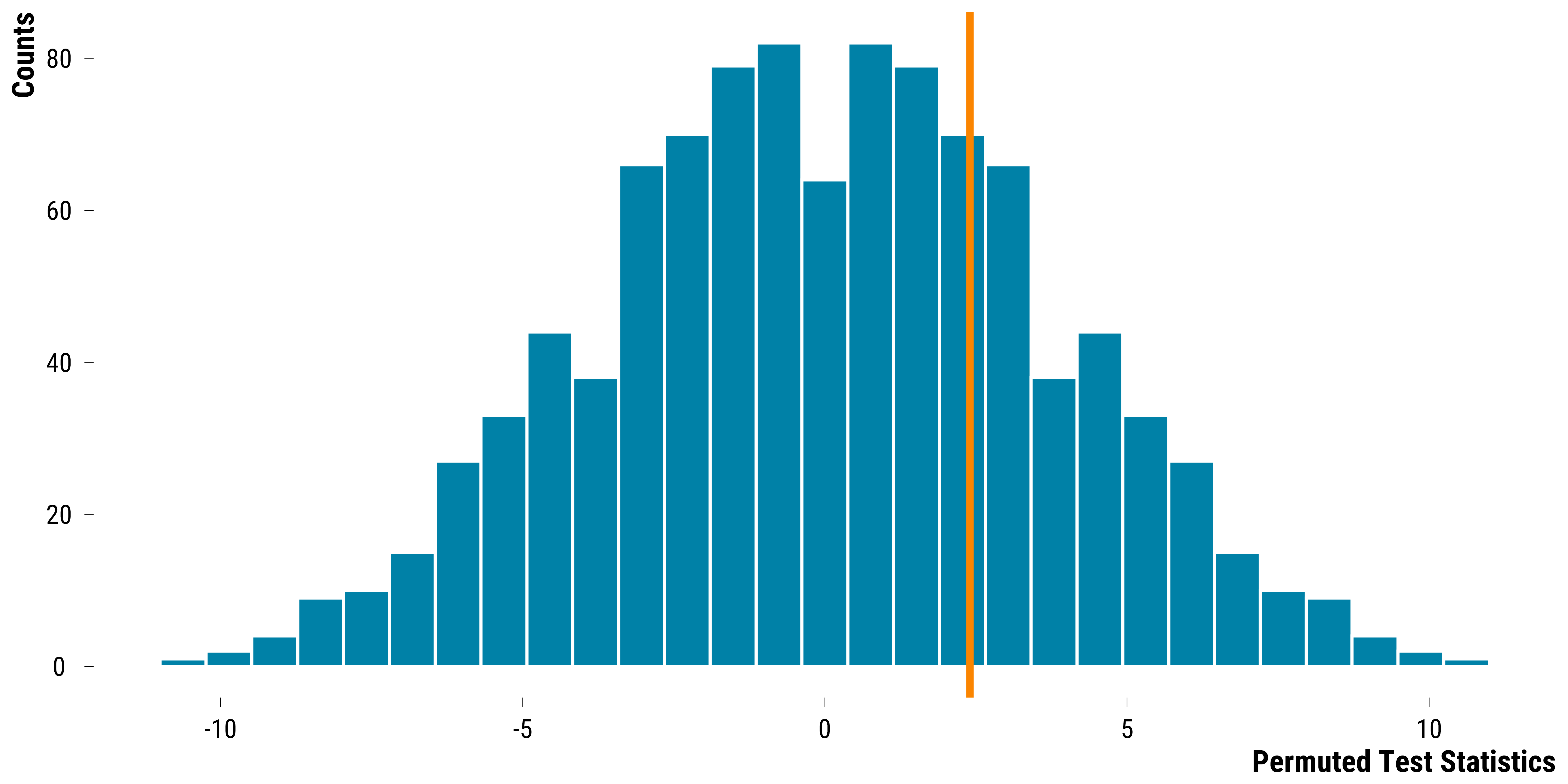
We plot below the distribution of the test statistic under the sharp null hypothesis:

Please show me the code!

# make the graph
graph_distribution_test_statistic <-
  tibble(distribution_test_statistics = distribution_test_statistics) %>%
  ggplot(., aes(x = distribution_test_statistics)) +
  geom_histogram(colour = "white", fill = my_blue) +
  geom_vline(xintercept = average_observed_pair_differences,
             size = 1.2,
             colour = my_orange) +
  xlab("Permuted Test Statistics") + ylab("Counts") +
  theme_tufte()

# display the graph
graph_distribution_test_statistic

Please show me the code!

# save the graph
ggsave(
  graph_distribution_test_statistic,
  filename = here::here(
    "inputs",
    "3.outputs",
    "3.toy_example",
    "distribution_test_statistic_sharp_null.pdf"
  ),
  width = 20,
  height = 10,
  units = "cm",
  device = cairo_pdf
)

Computing the Two-Sided P-Value

To compute a two-sided p-value, we again follow the explanations provided by Paul Rosenbaum in the chapter II of his textbook:

1. We first compute the proportions of permuted test statistics that are lower and higher than the observed test statistic.
2. We then double the smallest proportion.
3. We take the minimum of its value and one. This give us the two-sided \(p\)-value.

We implement this procedure as follows:

# number of permutations
n_permutations <- 1024

# compute upper proportion
upper_p_value <-
  sum(distribution_test_statistics >= average_observed_pair_differences) /
  n_permutations

# compute lower proportion
lower_p_value <-
  sum(distribution_test_statistics <= average_observed_pair_differences) /
  n_permutations

# double the smallest proportion
double_smallest_proprotion <- min(c(upper_p_value, lower_p_value)) * 2

# take the minimum of this proportion and one
p_value <- min(double_smallest_proprotion, 1)

The two-sided p-value for the sharp null hypothesis of no effect is equal to 0.55. We fail to reject the sharp null hypothesis of no effect, despite having simulated a true constant effect of +3 \(\mu g/m^{3}\).

Computing a 95% Fisherian Intervals for a Range of Sharp Null Hypotheses

In addition to computing the sharp null hypothesis of no effect, we can make the randomization inference procedure more informative by computing also the range of constant effects consistent with the data (i.e., a Fisherian interval). We follow again the explanations provided by Tirthankar Dasguspta and Donald B. Rubin in their forthcoming textbook on experimental design: Experimental Design: A Randomization-Based Perspective.

Steps of the Procedure

Instead of gauging a null effect for all units, we test a set of sharp null hypotheses \(H_{0}^{k}\): Y\(_{i,j}\)(1) = Y\(_{i,j}\)(0) + \(\tau_{k}\) for k =1,\(\ldots\), and where \(\tau_{k}\) represents a constant unit-level treatment effect size.

We must therefore choose of set of constant treatment effects that we would like to test. Here, we test a set of 81 sharp null hypotheses of constant treatment effects ranging from -20 to +20 with increments of 0.5.

For each constant treatment effect , we compute the upper -value associated with the hypothesis \(H_{0}^{k}\): Y\(_{i,j}\)(1) - Y\(_{i,j}\)(0) \(>\) \(\tau_{k}\) and the lower -value \(H_{0}^{k}\): Y\(_{i,j}\)(1) - Y\(_{i,j}\)(0) \(<\) \(\tau_{k}\).

To test each hypothesis, we compute the distribution of the test statistic. The sequence of hypotheses \(H_{0}^{k}\): Y\(_{i,j}\)(1) - Y\(_{i,j}\)(0) \(>\) \(\tau_{k}\) forms an upper -value function of \(\tau\), \(p^{+}(\tau)\), while the sequence of alternative hypotheses \(H_{0}^{k}\): Y\(_{i,j}\)(1) - Y\(_{i,j}\)(0) \(<\) \(\tau_{k}\) makes a lower -value function, \(\tau\), \(p^{-}(\tau)\). To compute the bounds of the 100(1-\(\alpha\))% Fisherian interval, we solve \(p^{+}(\tau) = \frac{\alpha}{2}\) for \(\tau\) to get the lower limit and \(p^{-}(\tau) = \frac{\alpha}{2}\) for the upper limit. We set our \(\alpha\) significance level to 0.05 and thus compute 95% Fisherian intervals. This procedure allows us to get the range of treatment effects consistent with our data.

As a point estimate of a Fisherian interval, we take the observed value of our test statistic which is the average of pair differences in a pollutant concentration. For avoiding confusion, it is very important to note that our test statistic is an estimate for the individual-level treatment effect of an hypothetical experiment and not for the average treatment effect.

Computational Shortcut

For each hypothesis, we could impute the missing potential outcomes. Then, we would randomly allocate the treatment, express the observed outcome and finally compute the average of pair differences. Again, this is a cumbersome way to proceed. Instead, we use the computional shortcut provided by Paul Rosenbaum in his textbook.

• We start by making a sharp null hypothesis of a constant treatment effect \(\tau\) such that \(Y_{i,j}(1) = Y_{i,j}(0) + \tau\).
• For a pair i, recall that the observed pair difference in outcomes is \(D_{i} = (W_{i,1} - W_{i,2})(Y_{i,1} - Y_{i,2})\).
• Under the sharp hypothesis, we have \(D_{i} = (W_{i,1} - W_{i,2})((Y_{i,1} + \tau W_{i,1}) - (Y_{i,2} + \tau W_{i,2}))\).
• We rearrange the right-hand side expression and find that \(D_{i} = \tau + (W_{i,1} - W_{i,2})(Y_{i,1}(0) - Y_{i,2}(0))\)
• We have \(D_{i} - \tau = (W_{i,1} - W_{i,2})(Y_{i,1}(0) - Y_{i,2}(0))\). This equation means that the observed pair difference in outcomes minus the hypothesized treatment effect is equal to \(\pm(Y_{i,1}(0) - Y_{i,2}(0))\). We can therefore carry out the randomization inference procedure seen in the previous section from the vector of observed pair differences adjusted for the hypothesized treatment effect.

Implementation in R

We start by creating a nested tibble of our vector of observed pair differences with the set of constant treatment effect sizes we want to test:

# create a nested dataframe with
# the set of constant treatment effect sizes
# and the vector of observed pair differences
ri_data_fi <-
  tibble(observed_pair_differences = observed_pair_differences) %>%
  summarise(data_observed_pair_differences = list(observed_pair_differences)) %>%
  group_by(data_observed_pair_differences) %>%
  expand(effect = seq(from = -20, to = 20, by = 0.5)) %>%
  ungroup()

# display the nested table
ri_data_fi

# A tibble: 81 x 2
   data_observed_pair_differences effect
   <list>                          <dbl>
 1 <dbl [10]>                      -20  
 2 <dbl [10]>                      -19.5
 3 <dbl [10]>                      -19  
 4 <dbl [10]>                      -18.5
 5 <dbl [10]>                      -18  
 6 <dbl [10]>                      -17.5
 7 <dbl [10]>                      -17  
 8 <dbl [10]>                      -16.5
 9 <dbl [10]>                      -16  
10 <dbl [10]>                      -15.5
# ... with 71 more rows

We then subtract for each pair difference the hypothetical constant effect:

# function to get the observed statistic
adjusted_pair_difference_function <-
  function(data_observed_pair_differences, effect) {
    adjusted_pair_difference <- data_observed_pair_differences - effect
    return(adjusted_pair_difference)
  }

# compute the adjusted pair differences
ri_data_fi <- ri_data_fi %>%
  mutate(
    data_adjusted_pair_difference = map2(
      data_observed_pair_differences,
      effect,
      ~ adjusted_pair_difference_function(.x, .y)
    )
  )

# display the table
ri_data_fi

# A tibble: 81 x 3
   data_observed_pair_differences effect data_adjusted_pair_difference
   <list>                          <dbl> <list>                       
 1 <dbl [10]>                      -20   <dbl [10]>                   
 2 <dbl [10]>                      -19.5 <dbl [10]>                   
 3 <dbl [10]>                      -19   <dbl [10]>                   
 4 <dbl [10]>                      -18.5 <dbl [10]>                   
 5 <dbl [10]>                      -18   <dbl [10]>                   
 6 <dbl [10]>                      -17.5 <dbl [10]>                   
 7 <dbl [10]>                      -17   <dbl [10]>                   
 8 <dbl [10]>                      -16.5 <dbl [10]>                   
 9 <dbl [10]>                      -16   <dbl [10]>                   
10 <dbl [10]>                      -15.5 <dbl [10]>                   
# ... with 71 more rows

We compute the observed mean of adjusted pair differences:

# compute the observed mean of adjusted pair differences
ri_data_fi <- ri_data_fi %>%
  mutate(observed_mean_difference = map(data_adjusted_pair_difference, ~ mean(.))) %>%
  unnest(cols = c(observed_mean_difference)) %>%
  select(-data_observed_pair_differences) %>%
  ungroup()

# display the table
ri_data_fi

# A tibble: 81 x 3
   effect data_adjusted_pair_difference observed_mean_difference
    <dbl> <list>                                           <dbl>
 1  -20   <dbl [10]>                                        22.4
 2  -19.5 <dbl [10]>                                        21.9
 3  -19   <dbl [10]>                                        21.4
 4  -18.5 <dbl [10]>                                        20.9
 5  -18   <dbl [10]>                                        20.4
 6  -17.5 <dbl [10]>                                        19.9
 7  -17   <dbl [10]>                                        19.4
 8  -16.5 <dbl [10]>                                        18.9
 9  -16   <dbl [10]>                                        18.4
10  -15.5 <dbl [10]>                                        17.9
# ... with 71 more rows

We use the same function_randomization_distribution() to compute the randomization distribution of the test statistic for each hypothesized constant effect:

# randomization distribution function
# this function takes as inputs the vector of pair differences and the number of pairs
# and then compute the average pair difference according
# to the permuted treatment assignment
function_randomization_distribution <-
  function(data_adjusted_pair_difference, n_pairs) {
    randomization_distribution = NULL
    n_columns = dim(permutations_matrix)[2]
    for (i in 1:n_columns) {
      randomization_distribution[i] =  sum(data_adjusted_pair_difference * permutations_matrix[, i]) / n_pairs
    }
    return(randomization_distribution)
  }

We run the function:

# compute the test statistic distribution
ri_data_fi <- ri_data_fi %>%
  mutate(
    randomization_distribution = map(
      data_adjusted_pair_difference,
      ~ function_randomization_distribution(., n_pairs = 10)
    )
  )

# display the table
ri_data_fi

# A tibble: 81 x 4
   effect data_adjusted_pair_differ~ observed_mean_d~ randomization_d~
    <dbl> <list>                                <dbl> <list>          
 1  -20   <dbl [10]>                             22.4 <dbl [1,024]>   
 2  -19.5 <dbl [10]>                             21.9 <dbl [1,024]>   
 3  -19   <dbl [10]>                             21.4 <dbl [1,024]>   
 4  -18.5 <dbl [10]>                             20.9 <dbl [1,024]>   
 5  -18   <dbl [10]>                             20.4 <dbl [1,024]>   
 6  -17.5 <dbl [10]>                             19.9 <dbl [1,024]>   
 7  -17   <dbl [10]>                             19.4 <dbl [1,024]>   
 8  -16.5 <dbl [10]>                             18.9 <dbl [1,024]>   
 9  -16   <dbl [10]>                             18.4 <dbl [1,024]>   
10  -15.5 <dbl [10]>                             17.9 <dbl [1,024]>   
# ... with 71 more rows

We compute the lower and upper p-values functions:

# define the p-values functions
function_fisher_upper_p_value <-
  function(observed_mean_difference,
           randomization_distribution) {
    sum(randomization_distribution >= observed_mean_difference) / n_permutations
  }

function_fisher_lower_p_value <-
  function(observed_mean_difference,
           randomization_distribution) {
    sum(randomization_distribution <= observed_mean_difference) / n_permutations
  }

# compute the lower and upper one-sided p-values
ri_data_fi <- ri_data_fi %>%
  mutate(
    p_value_upper = map2_dbl(
      observed_mean_difference,
      randomization_distribution,
      ~ function_fisher_upper_p_value(.x, .y)
    ),
    p_value_lower = map2_dbl(
      observed_mean_difference,
      randomization_distribution,
      ~ function_fisher_lower_p_value(.x, .y)
    )
  )

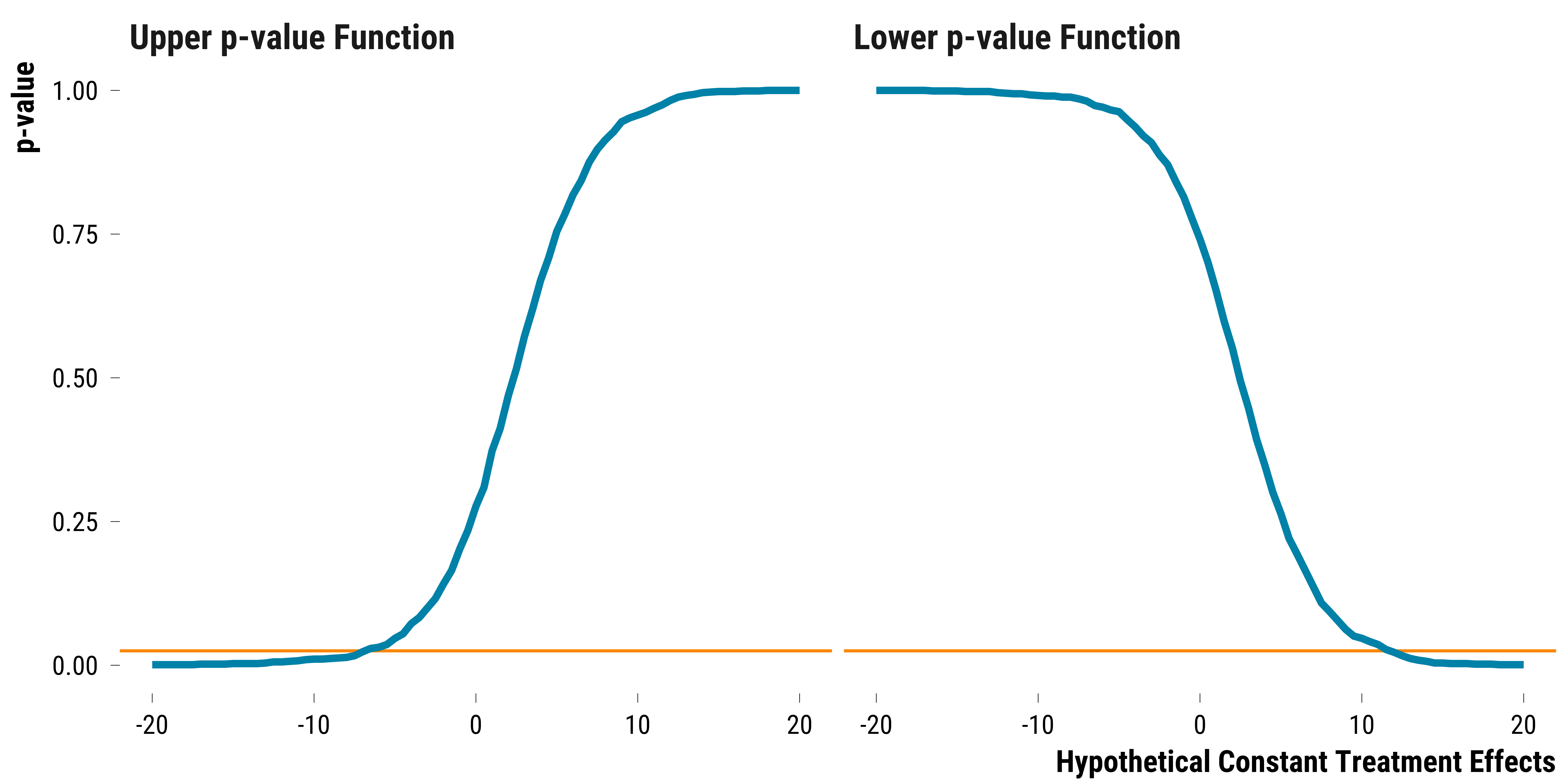
We plot below the lower and upper p-values functions:

Please show me the code!

# make the graph
graph_p_value_functions_sharp_nulls <- ri_data_fi %>%
  select(effect, p_value_upper, p_value_lower) %>%
  rename("Upper p-value Function" = p_value_upper,
         "Lower p-value Function" = p_value_lower) %>%
  pivot_longer(cols = -c(effect),
               names_to = "lower_upper",
               values_to = "p_value") %>%
  ggplot(., aes(x = effect, y = p_value)) +
  geom_hline(yintercept = 0.025, colour = my_orange) +
  geom_line(colour = my_blue, size = 1.2) +
  facet_wrap( ~ fct_rev(lower_upper)) +
  xlab("Hypothetical Constant Treatment Effects") + ylab("p-value") +
  theme_tufte()

# display the graph
graph_p_value_functions_sharp_nulls

Please show me the code!

# save the graph
ggsave(
  graph_p_value_functions_sharp_nulls,
  filename = here::here(
    "inputs",
    "3.outputs",
    "3.toy_example",
    "graph_p_value_functions_sharp_nulls.pdf"
  ),
  width = 20,
  height = 10,
  units = "cm",
  device = cairo_pdf
)

The orange line represents the alpha significance level, set at 5%, divided by two. We then retrieve the lower and upper bound of the 95% Fisherian interval:

# retrieve the constant effects with the p-values equal or the closest to 0.025
ri_data_fi <- ri_data_fi %>%
  mutate(
    p_value_upper = abs(p_value_upper - 0.025),
    p_value_lower = abs(p_value_lower - 0.025)
  ) %>%
  filter(p_value_upper == min(p_value_upper) |
           p_value_lower == min(p_value_lower)) %>%
  # in case two effect sizes have a p-value equal to 0.025, we take the effect size
  # that make the Fisherian interval wider to be conservative
  summarise(fi_lower_95 = min(effect),
            fi_upper_95 = max(effect))

As a point estimate, we take the value of the observed average of pair differences, that is to say 2.4 \(\mu g/m^{3}\). For this imaginary experiment, our point estimate is close to the true constant effect but the 95% Fisherian interval is wide: [-7, 11.5]. The data are consistent with both large negative and positive constant treatment effects.

Comparison with Neyman’s Approach

We can compare the result of the randomization inference procedure with the one we would obtain with Neyman’s approach. In that case, the inference procedure is built to target the average causal effect and the source of inference is both the randomization of the treatment and the sampling from a population. We can estimate the finite sample average effect, \(\tau_{\text{fs}}\), with the average of observed pair differences \(\hat{\tau}\):

\[\begin{equation*} \hat{\tau} = \frac{1}{I}\sum_{i=1}^J(Y^{\text{obs}}_{\text{t},i}-Y^{\text{obs}}_{\text{c},i}) = \overline{Y}^{\text{obs}}_{\text{t}} - \overline{Y}^{\text{obs}}_{\text{c}} \end{equation*}\]

Here, the subscripts \(t\) and \(c\) respectively indicate if the unit in a given pair is treated or not. \(I\) is the number of pairs. Since there are only one treated and one control unit within each pair, the standard estimate for the sampling variance of the average of pair differences is not defined. We can however compute a conservative estimate of the variance, as explained in chapter 10 of Imbens and Rubin (2015):

\[\begin{equation*} \hat{\mathbb{V}}(\hat{\tau}) = \frac{1}{I(I-1)}\sum_{I=1}^I(Y^{\text{obs}}_{\text{t},i}-Y^{\text{obs}}_{\text{c},i} - \hat{\tau})^{2} \end{equation*}\]

We finally compute an asymptotic 95% confidence interval using a Gaussian distribution approximation:

\[\begin{equation*} \text{CI}_{0.95}(\tau_{\text{fs}}) =\Big( \hat{\tau} - 1.96\times \sqrt{\hat{\mathbb{V}}(\hat{\tau})},\; \hat{\tau} + 1.96\times \sqrt{\hat{\mathbb{V}}(\hat{\tau})}\Big) \end{equation*}\]

As in the example of Imbens and Rubin (2015), we only have here 10 pairs. To build the 95% confidence interval, we use a \(t\)-distribution with degrees of freedom equal to I/2-1=9. The 0.975 quantile is equal to 2.262. We compute the 95% confidence interval with the following code:

# we store the number of pairs
n_pairs <- 10

# compute the standard error
squared_difference <-
  (observed_pair_differences - average_observed_pair_differences) ^ 2

# compute the standard error
standard_error <-
  sqrt(1 / (n_pairs * (n_pairs - 1)) * sum(squared_difference))

# compute the standard error
ci_lower_95 <-
  average_observed_pair_differences - qt(0.975, 9) * standard_error
ci_upper_95 <-
  average_observed_pair_differences + qt(0.975, 9) * standard_error

# store results
neyman_data_ci <-
  tibble(ci_lower_95 = ci_lower_95, ci_upper_95 = ci_upper_95)

The 95% confidence interval is equal to [-6.3, 11.1], which is very similar to the one found with randomization inference. However, this interval gives the range of average treatment effects consistent with the data.

Computing a 95% Fisherian Intervals For Weak Null Hypotheses

Finally, many researchers restrain from using randomization inference as a mode of inference since it assumes that treatment effects are constant across units. In most applications, this is arguably an unrealistic assumption. To overcome this limit, Jason Wu & Peng Ding (2021) propose to adopt a studentized test statistic that is finite-sample exact under sharp null hypotheses but also asymptotically conservative for the weak null hypothesis.

In the case of our toy example, this studentized test statistic is equal to the observed average of pair differences divided by the standard error of a pairwise experiment. We therefore just follow the same previous procedure but use the studentized statistic proposed by Jason Wu & Peng Ding (2021).

First, we create the data for testing a range of sharp null hypotheses:

# create a nested dataframe with 
# the set of constant treatment effect sizes
# and the vector of observed pair differences
ri_data_fi_weak <- tibble(observed_pair_differences = observed_pair_differences) %>%
  summarise(data_observed_pair_differences = list(observed_pair_differences)) %>%
  group_by(data_observed_pair_differences) %>%
  expand(effect = seq(from = -20, to = 20, by = 0.5)) %>%
  ungroup()

# display the nested table
ri_data_fi_weak

# A tibble: 81 x 2
   data_observed_pair_differences effect
   <list>                          <dbl>
 1 <dbl [10]>                      -20  
 2 <dbl [10]>                      -19.5
 3 <dbl [10]>                      -19  
 4 <dbl [10]>                      -18.5
 5 <dbl [10]>                      -18  
 6 <dbl [10]>                      -17.5
 7 <dbl [10]>                      -17  
 8 <dbl [10]>                      -16.5
 9 <dbl [10]>                      -16  
10 <dbl [10]>                      -15.5
# ... with 71 more rows

We then subtract for each pair difference the hypothetical constant effect using the previously used adjusted_pair_difference_function():

# compute the adjusted pair differences
ri_data_fi_weak <- ri_data_fi_weak %>%
  mutate(data_adjusted_pair_difference = map2(data_observed_pair_differences, effect, ~ adjusted_pair_difference_function(.x, .y)))

# display the table
ri_data_fi_weak

# A tibble: 81 x 3
   data_observed_pair_differences effect data_adjusted_pair_difference
   <list>                          <dbl> <list>                       
 1 <dbl [10]>                      -20   <dbl [10]>                   
 2 <dbl [10]>                      -19.5 <dbl [10]>                   
 3 <dbl [10]>                      -19   <dbl [10]>                   
 4 <dbl [10]>                      -18.5 <dbl [10]>                   
 5 <dbl [10]>                      -18   <dbl [10]>                   
 6 <dbl [10]>                      -17.5 <dbl [10]>                   
 7 <dbl [10]>                      -17   <dbl [10]>                   
 8 <dbl [10]>                      -16.5 <dbl [10]>                   
 9 <dbl [10]>                      -16   <dbl [10]>                   
10 <dbl [10]>                      -15.5 <dbl [10]>                   
# ... with 71 more rows

We then compute the observed studentized statistics:

# function to compute neyman t-statistic
function_neyman_t_stat <- function(pair_differences, n_pairs) {
  # compute the average of pair differences
  average_pair_difference <- mean(pair_differences)
  # compute the standard error
  squared_difference <-
    (pair_differences - average_pair_difference) ^ 2
  # compute the standard error
  standard_error <-
    sqrt(1 / (n_pairs * (n_pairs - 1)) * sum(squared_difference))
  # compute neyman t-statistic
  neyman_t_stat <- average_pair_difference / standard_error
  return(neyman_t_stat)
}


# compute the observed mean of adjusted pair differences
ri_data_fi_weak <- ri_data_fi_weak %>%
  mutate(
    observed_neyman_t_stat = map(
      data_adjusted_pair_difference,
      ~ function_neyman_t_stat(., n_pairs = 10)
    )
  ) %>%
  unnest(cols = c(observed_neyman_t_stat)) %>%
  select(-data_observed_pair_differences) %>%
  ungroup()

# display the table
ri_data_fi_weak

# A tibble: 81 x 3
   effect data_adjusted_pair_difference observed_neyman_t_stat
    <dbl> <list>                                         <dbl>
 1  -20   <dbl [10]>                                      5.82
 2  -19.5 <dbl [10]>                                      5.69
 3  -19   <dbl [10]>                                      5.56
 4  -18.5 <dbl [10]>                                      5.43
 5  -18   <dbl [10]>                                      5.30
 6  -17.5 <dbl [10]>                                      5.17
 7  -17   <dbl [10]>                                      5.04
 8  -16.5 <dbl [10]>                                      4.91
 9  -16   <dbl [10]>                                      4.78
10  -15.5 <dbl [10]>                                      4.65
# ... with 71 more rows

We create a function to carry out the randomization inference with the studentized test statistic:

# randomization distribution function
# this function takes the vector of pair differences
# and then compute the average pair difference according
# to the permuted treatment assignment
function_randomization_distribution_t_stat <-
  function(data_adjusted_pair_difference, n_pairs) {
    randomization_distribution = NULL
    n_columns = dim(permutations_matrix)[2]
    for (i in 1:n_columns) {
      # compute the average of pair differences
      average_pair_difference <-
        sum(data_adjusted_pair_difference * permutations_matrix[, i]) / n_pairs
      # compute the standard error
      squared_difference <-
        (data_adjusted_pair_difference - average_pair_difference) ^ 2
      # compute the standard error
      standard_error <-
        sqrt(1 / (n_pairs * (n_pairs - 1)) * sum(squared_difference))
      # compute neyman t-statistic
      randomization_distribution[i] = average_pair_difference / standard_error
    }
    return(randomization_distribution)
  }

We run the function:

# compute the test statistic distribution
ri_data_fi_weak <- ri_data_fi_weak %>%
  mutate(
    randomization_distribution = map(
      data_adjusted_pair_difference,
      ~ function_randomization_distribution_t_stat(., n_pairs = 10)
    )
  )

# display the table
ri_data_fi_weak

# A tibble: 81 x 4
   effect data_adjusted_pair_differ~ observed_neyman~ randomization_d~
    <dbl> <list>                                <dbl> <list>          
 1  -20   <dbl [10]>                             5.82 <dbl [1,024]>   
 2  -19.5 <dbl [10]>                             5.69 <dbl [1,024]>   
 3  -19   <dbl [10]>                             5.56 <dbl [1,024]>   
 4  -18.5 <dbl [10]>                             5.43 <dbl [1,024]>   
 5  -18   <dbl [10]>                             5.30 <dbl [1,024]>   
 6  -17.5 <dbl [10]>                             5.17 <dbl [1,024]>   
 7  -17   <dbl [10]>                             5.04 <dbl [1,024]>   
 8  -16.5 <dbl [10]>                             4.91 <dbl [1,024]>   
 9  -16   <dbl [10]>                             4.78 <dbl [1,024]>   
10  -15.5 <dbl [10]>                             4.65 <dbl [1,024]>   
# ... with 71 more rows

We compute the lower and upper p-values functions:

# define the p-values functions
function_fisher_upper_p_value <-
  function(observed_neyman_t_stat,
           randomization_distribution) {
    sum(randomization_distribution >= observed_neyman_t_stat) / n_permutations
  }

function_fisher_lower_p_value <-
  function(observed_neyman_t_stat,
           randomization_distribution) {
    sum(randomization_distribution <= observed_neyman_t_stat) / n_permutations
  }

# compute the lower and upper one-sided p-values
ri_data_fi_weak <- ri_data_fi_weak %>%
  mutate(
    p_value_upper = map2_dbl(
      observed_neyman_t_stat,
      randomization_distribution,
      ~ function_fisher_upper_p_value(.x, .y)
    ),
    p_value_lower = map2_dbl(
      observed_neyman_t_stat,
      randomization_distribution,
      ~ function_fisher_lower_p_value(.x, .y)
    )
  )

We plot below the lower and upper p-values functions:

Please show me the code!

# make the graph
graph_p_value_functions_weak_nulls <- ri_data_fi_weak %>%
  select(effect, p_value_upper, p_value_lower) %>%
  rename("Upper p-value Function" = p_value_upper, "Lower p-value Function" = p_value_lower) %>%
  pivot_longer(cols = -c(effect), names_to = "lower_upper", values_to = "p_value") %>%
  ggplot(., aes(x = effect, y = p_value)) +
  geom_hline(yintercept = 0.025, colour = my_orange) +
  geom_line(colour = my_blue, size = 1.2) +
  facet_wrap(~ fct_rev(lower_upper)) +
  xlab("Hypothetical Constant Treatment Effects") + ylab("p-value") +
  theme_tufte()

# display the graph
graph_p_value_functions_weak_nulls

Please show me the code!

# save the graph
ggsave(graph_p_value_functions_weak_nulls, filename = here::here("inputs", "3.outputs", "3.toy_example", "graph_p_value_functions_weak_nulls.pdf"), 
       width = 20, height = 10, units = "cm", device = cairo_pdf)

The orange line represents the alpha significance level, set at 5%, divided by two. We then retrieve the lower and upper bound of the 95% Fisherian interval:

# retrieve the constant effects with the p-values equal or the closest to 0.025
ri_data_fi_weak <- ri_data_fi_weak %>%
  mutate(
    p_value_upper = abs(p_value_upper - 0.025),
    p_value_lower = abs(p_value_lower - 0.025)
  ) %>%
  filter(p_value_upper == min(p_value_upper) |
           p_value_lower == min(p_value_lower)) %>%
  # in case two effect sizes have a p-value equal to 0.025, we take the effect size
  # that make the Fisherian interval wider to be conservative
  summarise(fi_lower_95 = min(effect),
            fi_upper_95 = max(effect))

The 95% Fisherian interval is equal to [-7, 11.5]. It is the same interval found with the randomization inference procedure using the average of pair differences as a test statistic. It is also very similar to the interval found with Neyman’s approach.